Result: Network unreachable (OS prevents it)

03 - Network Layer

Problem 1: Short Answer Questions

• (a) Why is it NOT possible to build a global network such as the Internet using just the link-layer (L2) switches?

  Solution

  In short: Link-layer switches forward frames based on MAC addresses, which are only meaningful on local network segments. Without the network layer’s IP addresses and routing, there’s no way to deliver packets across different networks globally.

  Elaboration:

  Limitations of Link-Layer Only:

  1. Scope of MAC Addresses

     • MAC addresses are meaningful only on the local network segment (LAN)
     • Switches use MAC address tables to forward frames to the correct port
     • MAC addresses change at each hop as packets traverse different links
     • Example: A packet from Host A to Host B on a distant network would need multiple different MAC addresses as it hops through switches

  2. No Inter-Network Routing

     • Switches have no concept of “networks” or “subnets”
     • They simply flood unknown MAC addresses to all ports (or use MAC address tables)
     • No way to intelligently route to distant parts of the network
     • Result: Inefficient use of bandwidth, poor scalability

  3. Broadcast Storm Problem

     • Without network-layer routing, switches would eventually flood all unknown traffic everywhere
     • Creates broadcast storms and network meltdowns
     • No way to limit the scope of flooding

  4. No Hierarchy

     • Link layer has no concept of network hierarchy or organization
     • Internet structure depends on nested routing domains (AS numbers, CIDR blocks)
     • Can’t organize billion-scale networks without hierarchical addressing

  Why Network Layer is Essential:

  • IP addresses are globally unique and hierarchical
  • Routers use IP to make intelligent routing decisions
  • Enables scalable, efficient global connectivity
  • Creates separate administrative domains (ASes, networks)

  Analogy: Link layer is like postal system within a building; network layer is the postal system connecting buildings, cities, countries.

• (b) Assume that the netmask for your network is 255.255.128.0 and your IPv4 address is 23.45.65.66. (1) What’s your IP subnet? (2) How many hosts can you connect to your IPv4 subnet?

  Solution

  In short: The IP subnet is 23.45.0.0, calculated by ANDing the IP with the netmask. You can connect 32,766 hosts (2^15 - 2), where 2^15 is the number of host bits available, minus 2 for network and broadcast addresses.

  Elaboration:

  Part 1: Finding the IP Subnet

  Given:

  • IPv4 address: 23.45.65.66
  • Netmask: 255.255.128.0

  Convert to binary:

  IP:       23.45.65.66
  Binary:   00010111.00101101.01000001.01000010
  Netmask:  255.255.128.0
  Binary:   11111111.11111111.10000000.00000000

  AND them together:

  IP AND Netmask:
  00010111.00101101.01000001.01000010
  11111111.11111111.10000000.00000000
  ═══════════════════════════════════════
  00010111.00101101.00000000.00000000
  = 23.45.0.0

  IP Subnet = 23.45.0.0/17

  (The /17 means 17 bits for network, 15 bits for host)

  Part 2: Number of Hosts

  • Host bits available: 32 - 17 = 15 bits
  • Total addresses: 2^15 = 32,768
  • Subtract 2:
    • 1 for network address (all host bits = 0): 23.45.64.0
    • 1 for broadcast address (all host bits = 1): 23.45.127.255
  • Usable hosts = 32,768 - 2 = 32,766

  Answer:

  1. IP Subnet: 23.45.0.0/17
  2. Maximum hosts: 32,766

• (c) What would be the disadvantage to placing the IP version number in a place other than the first byte of the IP header?

  Solution

  In short: The version number must be in the first byte so receiving nodes can immediately identify the IP version and parse the rest of the header correctly. Placing it elsewhere would require assuming a fixed header format, making it impossible to handle mixed IP versions efficiently.

  Elaboration:

  Why First Byte is Critical:

  The IP version field is in the first 4 bits of the first byte of the IP header. This is essential for:

  1. Immediate Recognition

     • Network devices can read the first byte without knowing the header length
     • Allows routers to identify if it’s IPv4, IPv6, or other version
     • If version were elsewhere, routers wouldn’t know how to parse the header

  2. Handling Mixed Versions

     • Networks may contain both IPv4 and IPv6 traffic simultaneously
     • First byte allows quick distinction without parsing entire packet
     • Example: A switch can immediately see version 4 or 6 and route accordingly

  3. Hardware Processing

     • Network interface cards (NICs) and switches process packets in order
     • They read the first byte to identify packet type before doing anything else
     • Placing version elsewhere would require buffering entire header first

  4. Backward Compatibility

     • IPv6 nodes can immediately recognize IPv4 packets and handle them differently
     • Can drop unsupported versions or route to gateways
     • Placing version elsewhere would break this capability

  Example Consequence of Bad Placement:

  If version were in byte 3 instead:

  • Router can’t know header length until reading byte 3
  • Can’t know if IP header is 20 bytes (IPv4) or 40 bytes (IPv6)
  • Would need to assume a fixed format, breaking extensibility
  • Can’t handle version transitions gracefully

  Conclusion: Early position (first byte, first 4 bits) is a fundamental design requirement for IP protocols.

• (d) Give a network application that would be better suited for a datagram-based network than a virtual-circuit-oriented network and a network application that would be better suited for a virtual-circuit-oriented network than a datagram-based network. Justify your answer!

  Solution

  In short: DNS queries are ideal for datagrams (simple request-response, low overhead, stateless). Video conferencing is ideal for virtual circuits (requires ordered delivery, predictable latency, QoS guarantees). The choice depends on whether the application needs connection state or just simple message exchange.

  Elaboration:

  Application Better for Datagram Networks: DNS Query

  Why DNS suits datagrams:

  1. Simple request-response pattern

     • Client sends single DNS query (datagram)
     • Server sends back single response (datagram)
     • No connection state needed

  2. Stateless

     • Each query is independent
     • Server doesn’t need to remember previous queries
     • No connection setup overhead

  3. Low overhead

     • No connection establishment (3-way handshake)
     • No connection teardown
     • Minimal latency impact

  4. Fault tolerance

     • If response lost, client retransmits query
     • No connection state to clean up on failures
     • Simple timeout-based recovery

  Example: User types domain name → DNS client sends single datagram → DNS server responds with single datagram.

  Application Better for Virtual Circuit Networks: Video Conferencing

  Why video conferencing suits virtual circuits:

  1. Ordered delivery essential

     • Video frames must arrive in order
     • Out-of-order frames create artifacts and jumps
     • Virtual circuits guarantee ordering

  2. Predictable latency

     • Human conversation requires consistent round-trip time
     • Variable latency (jitter) is annoying in video calls
     • Virtual circuits maintain consistent path → predictable delay

  3. Resource reservation

     • Video requires sustained bandwidth (e.g., 2-5 Mbps)
     • Virtual circuits can reserve bandwidth along the path
     • Ensures call quality won’t degrade due to congestion

  4. Connection state useful

     • Conference participants form a logical group
     • Connection state reflects active participants
     • Dropping connection cleanly ends conference

  Example: Alice calls Bob → establish virtual circuit → reserve bandwidth → transmit video frames in order with guaranteed quality.

  Summary Comparison:

  Aspect	DNS (Datagram)	Video Conference (VC)
  Duration	Milliseconds	Minutes/hours
  State needed	None	Connection state
  Order critical	No	Yes
  QoS needed	No	Yes
  Setup overhead	Bad if needed	Good for long calls
  Flexibility	Good (any server)	Bad (fixed path)

• (e) Consider a network that uses virtual circuits. Is it possible for 2 packets to arrive out of order at the destination? Why or why not?

  Solution

  In short: No, packets cannot arrive out of order in a virtual circuit network. The VC establishes a fixed path through the network, and all packets follow the same path with identical propagation and transmission characteristics, guaranteeing in-order delivery.

  Elaboration:

  Virtual Circuit Characteristics:

  1. Fixed Path Established

     • When a virtual circuit is set up, a specific path through the network is chosen
     • Example path: Source → Router A → Router B → Router C → Destination
     • All packets in the VC follow this exact same path

  2. Identical Timing Characteristics

     • All packets on the same VC experience:
       • Same propagation delays (same physical path)
       • Same transmission delays (same links)
       • Same queuing behavior (reserved resources)
     • If packet 1 arrives at Router A at time T, packet 2 arrives at time T+Δ
     • These time differences are preserved at each hop

  3. In-Order Guarantee

     • Packet 1 sent before Packet 2
     • Both take the same path at the same speed
     • Packet 1 arrives at destination before Packet 2
     • Ordering is mathematically guaranteed

  Why Datagrams Can Arrive Out-of-Order:

  In contrast, datagram networks (like IP) can deliver out-of-order because:

  • Different packets can take different routes
  • Route changes can cause different propagation delays
  • Different queuing at intermediate routers
  • Example: Packet 2 finds empty route while Packet 1 hits congestion

  Analogy:

  • Virtual Circuit: Passengers on same train car always arrive in order
  • Datagram: Passengers on different trains might arrive in different orders

  Conclusion: In-order delivery is a guaranteed property of virtual circuit networks, not a coincidence.

• (f) The Internet is running out of IPv4 addresses to assign, but there are substantially less than four billion hosts on the Internet. Briefly explain why this is happening.

  Solution

  In short: IPv4 addresses are exhausted due to inefficient allocation (Class A/B networks assigned wastefully), NAT limitations, reserved address blocks, fragmentation, and infrastructure devices consuming addresses. Not all 2^32 addresses are available for hosts.

  Elaboration:

  Why IPv4 is Exhausted Despite Only Billions of Hosts:

  1. Reserved Address Blocks

     • **(224)**0.0.0 - **(255)**255.255.255: Multicast and reserved (25% of address space!)
     • **(127)**0.0.0/8: Loopback (16 million addresses)
     • **(169)**254.0.0/16: Link-local (65,000 addresses)
     • **(10)**0.0.0/8, 172.16.0.0/12, 192.168.0.0/16: Private (non-routable)
     • Result: ~2 billion addresses unavailable for public use

  2. Inefficient Class-Based Allocation (before CIDR)

     • Class A networks: Each company got /8 (16 million addresses)
     • Example: MIT has 18.0.0.0/8, Apple has 17.0.0.0/8
     • Many Class A holders use only small fraction of allocated addresses
     • Once allocated, extremely difficult to reclaim

  3. Infrastructure Device Addresses

     • Routers, switches, servers consume addresses
     • Each interface on a router needs an address
     • Data centers with millions of servers need millions of addresses
     • Cloud infrastructure (AWS, Google Cloud) reserve large blocks

  4. Subnetting Overhead

     • Each subnet wastes 2 addresses (network and broadcast)
     • Aggregation/fragmentation leads to inefficient allocation
     • Multiple small subnets waste more addresses per host

  5. Address Hoarding

     • Organizations request more than needed (uncertainty)
     • ISPs reserve blocks for future growth
     • No easy way to reclaim unused addresses

  6. NAT Limitations

     • NAT allows multiple hosts behind one public IP
     • But NAT has limitations (breaks some protocols, adds complexity)
     • Not a complete solution for unlimited growth

  Timeline:

  • IPv4 exhaustion predictions: Made since 1990s
  • IANA pool exhausted: 2011
  • Regional registries starting to run out: 2012-2015
  • RIRs now rationing addresses

  Solutions in Deployment:

  • IPv6 (340 undecillion addresses!)
  • NAT (temporary workaround)
  • Address conservation techniques
  • Secondary markets for buying/selling addresses

• (g) What is CIDR (Classless Inter Domain Routing)? Briefly explain.

  Solution

  In short: CIDR eliminates the rigid Class A/B/C system, allowing arbitrary network/host bit divisions specified by a prefix length (e.g., 192.168.1.0/24). This enables more efficient IP address allocation and routing aggregation.

  Elaboration:

  The Class System Problem:

  Before CIDR, IPv4 addresses were divided into rigid classes:

  • Class A (/8): 1 network bit, 24 host bits (16 million hosts per network)
  • Class B (/16): 2 network bits, 16 host bits (65,000 hosts per network)
  • Class C (/24): 3 network bits, 8 host bits (254 hosts per network)

  Problem: Many organizations needed more than 254 hosts but much less than 65,000. Allocating a Class B wasted ~60,000 addresses.

  CIDR Solution:

  CIDR allows arbitrary prefix lengths using notation: IP_Address/prefix_length

  Examples:

  • **(192)**168.1.0/25: 7 host bits (128 hosts)
  • **(10)**0.0.0/22: 10 host bits (1024 hosts)
  • **(172)**16.0.0/12: 12 host bits (4096 hosts)

  Key Benefits:

  1. Efficient Allocation

     • Organizations get exactly what they need
     • If you need 1000 hosts, get /22 instead of /16
     • Saves millions of addresses

  2. Route Aggregation

     • Multiple networks can be aggregated into single routing entry
     • Example: Routes for 192.168.0.0/24 through 192.168.3.0/24 aggregate to 192.168.0.0/22
     • Reduces routing table size dramatically

  3. Supernetting

     • Can combine multiple traditional Class C networks
     • **(192)**168.0.0/24 + 192.168.1.0/24 + 192.168.2.0/24 + 192.168.3.0/24 = 192.168.0.0/22

  CIDR Notation Breakdown:

  192.168.1.0/24
  ├─ 192.168.1.0: Network address
  └─ /24: First 24 bits are network, last 8 bits are host

  Historical Impact:

  • Introduced: 1993 (RFC 1518, 1519)
  • Replaced: Classful routing
  • Result: Extended IPv4 life by at least 10-15 years
  • Enabled: More efficient routing and address allocation

  Note: CIDR is fundamental to modern IP routing and addressing.

• (h) The IPv6 header is 40 bytes long, as opposed to 20 bytes of IPv4 header, while the address size has quadrupled. What functionality has disappeared from the fixed header?

  Solution

  In short: IPv6 removed several IPv4 header fields: checksum (verified at lower/higher layers), flags/fragment fields (handled via extension headers), and options (moved to extension headers). IPv6 also removed TTL (replaced with Hop Limit) and simplified header alignment, trading fixed header simplicity for extension header flexibility.

  Elaboration:

  IPv4 Header Fields (~20 bytes):

  Version | IHL | DSCP | ECN | Total Length
  Flags | Fragment Offset
  TTL | Protocol | Checksum
  Source IP (4 bytes)
  Destination IP (4 bytes)
  Options (variable)

  IPv6 Header Fields (40 bytes):

  Version | Traffic Class | Flow Label
  Payload Length | Next Header | Hop Limit
  Source IP (16 bytes)
  Destination IP (16 bytes)
  [Extension headers follow, not in fixed header]

  What Disappeared:

  1. Checksum Field (REMOVED)

     • IPv4: 2 bytes for header checksum
     • IPv6: NO checksum in IP header
     • Rationale:
       • Link layer (Ethernet CRC) catches transmission errors
       • Transport layer (TCP/UDP checksums) validate end-to-end
       • IP checksum recalculation at each hop is expensive
       • Modern networks have better error checking at L2/L4

  2. Fragmentation Fields (MOVED)

     • IPv4: Flags (3 bits) + Fragment Offset (13 bits) = 2 bytes
     • IPv6: NO fragmentation in header, uses Extension Headers
     • Rationale:
       • Source host does fragmentation before sending (if needed)
       • Routers never fragment IPv6 packets
       • Eliminates router processing overhead
       • Routers send ICMP “Packet Too Big” instead

  3. IHL Field (SIMPLIFIED)

     • IPv4: IHL (4 bits) specifies header length (due to options)
     • IPv6: Fixed 40-byte header, no variable length
     • Rationale:
       • Simplifies parsing and hardware processing
       • Options moved to Extension Headers (optional, come after main header)

  4. Options (MOVED)

     • IPv4: Options field (variable, up to 40 bytes)
     • IPv6: Extension Headers (separate, optional)
     • Rationale:
       • Optional features don’t belong in required header
       • Routers can skip unrecognized extension headers
       • More flexible than IPv4 options

  5. TTL → Hop Limit (RENAMED, SAME SIZE)

     • IPv4: TTL (8 bits)
     • IPv6: Hop Limit (8 bits)
     • Functionally identical, just renamed

  Why IPv6 Header is Larger Despite Removals:

  • IPv4 addresses: 4 bytes each × 2 = 8 bytes
  • IPv6 addresses: 16 bytes each × 2 = 32 bytes
  • Address growth (24 bytes) > Field removals (2-4 bytes)
  • Result: Net gain of 20 bytes

  IPv6 Design Philosophy:

  “Simplify the main header, put optional features in extension headers”

  This makes IPv6 routers much faster because they process a fixed-size header without dealing with optional fields.

• (i) How many bits does an IPv4 address have? What is an IP subnet?

  Solution

  In short: IPv4 addresses are 32 bits long (4 bytes). An IP subnet is a contiguous block of IP addresses where the first N bits are the network address and the remaining (32-N) bits are host addresses, typically written as network_address/N (CIDR notation).

  Elaboration:

  IPv4 Address Size:

  • Total bits: 32 bits
  • Written as: 4 octets (bytes) in dotted decimal
  • Range: 0.0.0.0 to 255.255.255.255 (2^32 = 4,294,967,296 addresses)
  • Example: 192.168.1.100

  IP Subnet Definition:

  An IP subnet is a logical subdivision of an IP network where:

  • A contiguous block of consecutive IP addresses
  • Divided into network bits (prefix) and host bits (suffix)
  • All hosts on the same subnet have the same network bits

  Subnet Notation (CIDR):

  192.168.1.0/24
  ├─ 192.168.1.0: Network address
  ├─ /24: Prefix length (24 bits for network, 8 bits for host)
  ├─ 255.255.255.0: Netmask (alternative representation)
  └─ Usable hosts: 254 (256 - 2 for network and broadcast)

  Subnet Example:

  Subnet: 192.168.1.0/24

  • Network address: 192.168.1.0 (when host bits = 0)
  • Broadcast address: 192.168.1.255 (when host bits = 1)
  • First usable host: 192.168.1.1
  • Last usable host: 192.168.1.254
  • Subnet mask: 255.255.255.0
  • Number of addresses: 256 (2^8)
  • Usable hosts: 254

  How Subnets Work:

  1. Same Subnet = Direct Link

     • If two IPs share the same network bits → on same subnet
     • Can communicate directly via link layer (MAC addresses)
     • No router needed

  2. Different Subnet = Routing Needed

     • Different network bits → different subnets
     • Must communicate via routers
     • Routers strip old MAC header, add new one for each hop

  Subnet Calculation Example:

  IP: 10.20.30.50/16

  • Network bits: 10.20 (first 16 bits)
  • Host bits: 30.50 (last 16 bits)
  • Subnet: 10.20.0.0/16
  • Maximum hosts: 2^16 - 2 = 65,534

• (j) How many bits does an IPv6 address have? How many bits are used for interface id?

  Solution

  In short: IPv6 addresses are 128 bits long. The last 64 bits are used for the Interface ID (host portion), while the first 64 bits are the network prefix. This matches IPv4’s /64 subnet standard used in most IPv6 deployments.

  Elaboration:

  IPv6 Address Size:

  • Total bits: 128 bits (16 bytes)
  • Written as: 8 groups of 4 hexadecimal digits, separated by colons
  • Range: 2^128 = 340,282,366,920,938,463,463,374,607,431,768,211,456 addresses
  • Example: 2001:0db8:85a3:0000:0000:8a2e:0370:7334

  IPv6 Address Structure:

  Standard /64 Subnet:

  2001:db8:85a3:0000 : 0000:8a2e:0370:7334
  └─ First 64 bits (Network prefix)  └─ Last 64 bits (Interface ID)

  Bit Breakdown:

  Component	Bits	Purpose
  Network Prefix	64	Routing and organization
  Interface ID	64	Host identifier on that network

  Why 64 Bits for Interface ID:

  1. Sufficient for Any Need

     • 2^64 = 18 quintillion possible host IDs
     • More than enough for any subnet
     • Far exceeds any practical need

  2. Auto-Configuration Support

     • 64-bit Interface ID can be auto-generated from MAC address
     • MAC address (48 bits) can be expanded to 64 bits (EUI-64 format)
     • Enables SLAAC (Stateless Address Auto-Configuration)

  3. Simplified Routing

     • All subnets are /64
     • Routers don’t need VLSM (Variable Length Subnet Masking)
     • Standardization improves performance

  IPv6 Prefix Conventions:

  • /32: Typical allocation to ISP or large organization
  • /48: Regional registry allocation
  • /56: Typical allocation to small organization or customer
  • /64: Standard subnet size (for hosts)
  • /128: Single host (loopback, anycast)

  Example Breakdown:

  Address: 2001:db8:85a3::1/64

  • Network: 2001:db8:85a3:0000::/64
  • Interface ID: 0000:0000:0000:0001
  • This host is on subnet 2001:db8:85a3::/64 with ID 1

  Comparison with IPv4:

  Aspect	IPv4	IPv6
  Total bits	32	128
  Network bits	Variable (8-30)	Typically 64
  Host bits	Variable (2-24)	64
  Subnets per /64	N/A	1 (standard)

  Note: While /64 is standard, IPv6 supports any prefix length (e.g., /32, /48, /56, /128) for different purposes.

• (k) List 2 reasons why an organization might have assigned private IPv4 addresses to its hosts.

  Solution

  In short: Organizations use private IPv4 addresses to enable internal communication without consuming public IP addresses, and to provide network isolation and security by hiding internal network topology from the internet. Private addresses (10.0.0.0/8, 172.16.0.0/12, 192.168.0.0/16) are not routable on the public internet.

  Elaboration:

  Reason 1: IP Address Conservation

  • Public IPv4 addresses are scarce and expensive

    • Each public address costs money and requires allocation
    • ISPs charge for large address blocks

  • Private addresses are unlimited and free

    • RFC 1918 reserves three address ranges:
      • **(10)**0.0.0/8 (16 million addresses)
      • **(172)**16.0.0/12 (1 million addresses)
      • **(192)**168.0.0/16 (65,000 addresses)
    • Any organization can use these internally

  • Enables many hosts with few public IPs

    • 1000-person company needs 1000 private IPs internally
    • But might only need 10-50 public IPs via NAT gateway
    • NAT translates private→public for outbound traffic

  Reason 2: Network Security and Isolation

  • Hidden topology

    • External attackers can’t scan internal network directly
    • Can only see public IPs of NAT gateways
    • Internal subnet structure hidden from internet

  • Firewall benefits

    • NAT gateway acts as security barrier
    • Internal hosts protected from unsolicited inbound connections
    • Easier to implement perimeter security with one public IP

  • Prevents internal address scanning

    • External hosts can’t directly probe 192.168.x.x
    • Private address space is invisible to internet routers
    • Adds layer of obscurity-based security

  • Control and monitoring

    • All internal-to-external traffic goes through NAT
    • Can monitor and log all outbound connections
    • Easier to enforce security policies at single gateway

  Practical Example:

  Company with 500 employees:

  • Internal network: 192.168.0.0/16 (65,536 private addresses)
  • Public connection: 203.45.67.100 (1 public address)
  • NAT gateway: Translates all internal traffic to the public address
  • External internet sees: 203.45.67.100 (can’t see 500 internal IPs)
  • Cost saved: ~500 public addresses not needed

  Additional Benefits:

  • Enables flexible internal network redesign without ISP coordination
  • Supports multiple networks with overlapping private addresses
  • Works across organizational mergers (no address collision issues)

• (l) What’s a Link Local IPv4 address. What is it used for?

  Solution

  In short: Link-Local IPv4 addresses (169.254.0.0/16) are automatically assigned when DHCP fails or is unavailable. They enable communication only on the local network segment, useful for device discovery and bootstrap when no DHCP server is present.

  Elaboration:

  Link-Local IPv4 Address Definition:

  • Address range: 169.254.0.0/16 (169.254.0.1 to 169.254.255.254)
  • Scope: Local network segment only (not routable)
  • Standard: RFC 3927 (IPv4 Link-Local)
  • Automatic assignment: Triggered when DHCP fails

  How Link-Local Assignment Works:

  1. Host boots up and attempts DHCP

  2. No DHCP response received (server down or unavailable)

  3. Host self-assigns address from 169.254.0.0/16

     • Randomly selects address
     • Checks with ARP if already in use
     • If used, picks another random address
     • This is called APIPA (Automatic Private IP Addressing)

  4. Host can now communicate with other hosts on same segment

  5. If DHCP becomes available later, can request proper address

  What Link-Local Addresses Are Used For:

  1. Bootstrap and Device Discovery

     • When device first boots with no DHCP server
     • Can discover and communicate with other devices on segment
     • Enables peer-to-peer communication

  2. Network Device Setup

     • Network switches, routers, printers can be accessed
     • Admin can connect laptop with 169.254.x.x address
     • Configure device before assigning permanent address

  3. Fallback Connectivity

     • Network still functions locally if DHCP fails
     • Devices can still communicate with each other
     • Graceful degradation instead of no connectivity

  4. Ad-hoc Networking

     • Two devices connected directly can both self-assign link-local
     • Enable communication without infrastructure
     • Example: Two computers connected via single cable

  Limitations:

  • Not routable

    • Routers discard packets with 169.254.x.x as destination
    • Cannot reach beyond local segment
    • No internet connectivity

  • No DNS resolution

    • Not registered in DNS
    • Cannot use domain names with link-local IPs

  • Temporary solution

    • Not meant for permanent addressing
    • Should be replaced with DHCP when available

  IPv6 Equivalent:

  IPv6 has a similar concept: Link-Local IPv6 addresses (fe80::/10)

  • Automatically assigned to every IPv6 interface
  • Used for local communication (ARP equivalent, router discovery)
  • Every IPv6 host gets both link-local and global address

  Practical Example:

  Network admin wants to configure a new switch:

  1. Connect laptop via Ethernet
  2. Laptop fails to get DHCP (no DHCP server yet)
  3. Laptop self-assigns 169.254.44.50
  4. Switch also self-assigns 169.254.88.80 (from APIPA)
  5. Admin can ping and SSH to 169.254.88.80
  6. Admin configures switch with permanent address
  7. Admin assigns DHCP pool
  8. Laptop now gets real address from DHCP

• (m) What’s a loopback IPv4 address. Is it possible for a packet sent to the loopback IPv4 address to leave the host and sent over the network?

  Solution

  In short: Loopback addresses (127.0.0.1 to 127.255.255.255) allow a host to send packets to itself for testing. Packets sent to loopback are never transmitted on the network—they’re processed entirely within the host’s IP stack, never reaching the link layer.

  Elaboration:

  Loopback Address Definition:

  • Address range: 127.0.0.0/8 (127.0.0.1 to 127.255.255.255)
  • Standard: 127.0.0.1 is most common
  • Scope: Local machine only (special, non-routable)
  • Uses: Testing, local inter-process communication

  How Loopback Works:

  When a host sends a packet to loopback address:

  1. IP stack recognizes loopback address

     • Special handling in IP layer
     • Never passed to link layer (Ethernet, etc.)

  2. Packet is delivered locally

     • Packet processed as if received from network
     • Delivered to appropriate transport layer (TCP/UDP)
     • Application receives data

  3. No transmission occurs

     • Packet never hits network interface
     • No Ethernet frame created
     • Nothing transmitted on wire
     • No router involvement

  Packet Path for Loopback:

  Application → Transport (TCP/UDP) → IP Layer
               ↓
          [Loopback detected]
               ↓
          [Packet delivered back up]
               ↓
          Transport (TCP/UDP) → Application

  Packet Path for Normal Destination:

  Application → Transport → IP → Link Layer → Ethernet → Network

  Common Loopback Uses:

  1. Testing without network

     • Test application without networking hardware
     • Useful for development and debugging
     • No network issues can interfere

  2. Local inter-process communication

     • Process A listens on 127.0.0.1:8080
     • Process B connects to 127.0.0.1:8080
     • Useful for IPC (Inter-Process Communication)
     • Example: Web browser → localhost:8080 web server

  3. Service testing

     $ curl http://127.0.0.1:80
     $ telnet localhost 22

  Can Loopback Packets Leave the Host?

  NO - Explicitly impossible:

  1. IP layer enforces loopback scope

     • IP stack has special case for 127.0.0.0/8
     • Routers also reject loopback addresses
     • If somehow escaped, routers would discard it

  2. No routing possible

     • Loopback addresses not in routing tables
     • Can’t be source or destination for routable packets
     • By design, purely local

  3. Layer 2 never involved

     • Packets never reach Ethernet/link layer
     • No MAC address translation (ARP) occurs
     • Link-layer is completely bypassed

  Example Proof:

  Try to ping another machine using loopback source:

  $ ping -I 127.0.0.1 8.8.8.8
  # Result: Network unreachable (OS prevents it)

  The OS kernel refuses to send packets with 127.x.x.x as source or destination.

  Why This Design:

  • Safety: Prevents accidental loopback traffic on network
  • Performance: No overhead of network transmission for local testing
  • Clarity: Clear distinction between local and remote services
  • Security: Loopback services aren’t exposed to network

  IPv6 Equivalent:

  IPv6 loopback: ::1 (single address in 128-bit form)

  • Same concept and behavior
  • Only address in ::1/128 range

• (n) Explain why IPv4 does reassembly at the destination rather than at the routers.

  Solution

  In short: Reassembly at the destination is more efficient because routers would need to maintain reassembly buffers for every flow, creating memory overhead and complexity. Destination reassembly is simpler—the final host has all the time needed to reassemble fragments. If reassembly failed at a router, all downstream traffic would be delayed, whereas destination-side reassembly only affects that one connection.

  Elaboration:

  Why Not Reassemble at Routers:

  1. Memory and State Overhead

     • Routers would need reassembly buffers for every packet flow passing through
     • A busy router handling millions of flows would need gigabytes of memory
     • State management becomes complex: tracking which fragments belong to which flow
     • Slows down router throughput (primary job is routing, not reassembly)

  2. Fragmentation at Each Hop

     • If router reassembles, then fragments again for smaller MTU downstream
     • Results in multiple fragmentation/reassembly cycles
     • Wastes CPU and memory on repeated work
     • No benefit over single reassembly at destination

  3. Complexity and Delay

     • Routers would need to wait for all fragments before forwarding
     • Waiting time introduces latency
     • Router must decide when fragment loss occurred (timeout mechanism)
     • More moving parts = more opportunities for failure

  4. Path Changes

     • If route changes mid-reassembly, router has incomplete data
     • Would need to flush buffers or retransmit fragments
     • Complicates routing protocol interactions

  Why Destination Reassembly is Better:

  1. Destination has all the time

     • Final host receives fragments as they arrive
     • Can buffer them indefinitely (host memory >> router memory)
     • No deadline pressure to reassemble

  2. Simple design

     • End-to-end principle: let hosts handle complexity
     • Routers remain simple and fast
     • Follows Unix philosophy: do one thing well

  3. One reassembly per packet

     • Packet fragmented once at source
     • Reassembled once at destination
     • No intermediate reassembly/re-fragmentation cycles

  4. Clean failure mode

     • If one fragment lost: only that connection affected
     • If router reassembly failed: could affect all downstream traffic
     • Destination can timeout and request retransmission via TCP

  Example:

  Source → Router A (MTU 1500) → Router B (MTU 1000) → Router C (MTU 1500) → Destination

  Router Reassembly Model:

  • Source sends 1500-byte packet
  • Router B must reassemble, then re-fragment for 1000 MTU
  • Reassemble again at Router C for 1500 MTU
  • (Wasteful!)

  Destination Reassembly Model:

  • Source fragments for smallest MTU (1000) at start
  • All routers forward fragments directly
  • Destination reassembles once
  • (Efficient!)

• (o) Explain the difference between how IPv4 and IPv6 handle passing packets through sub-networks with MTU (Maximum Transmission Units) smaller than the originating sub-network could handle. Make sure to explain the advantages of each approach.

  Solution

  In short: IPv4 routers fragment packets at intermediate hops if MTU is smaller than the packet size, whereas IPv6 source hosts must discover the path MTU beforehand and fragment at the source. IPv6’s approach avoids router fragmentation overhead but requires source-side path MTU discovery mechanism. IPv4’s approach is simpler for sources but burdens routers.

  Elaboration:

  IPv4 Fragmentation (Router-based):

  How it works:

  1. Source sends packet sized for its local MTU (e.g., 1500 bytes)
  2. Router receives packet destined for network with smaller MTU (e.g., 1000 bytes)
  3. Router fragments the packet into smaller pieces
  4. Each fragment has its own IP header, maintains same ID for reassembly
  5. Destination reassembles fragments into original packet

  IPv4 Advantages:

  • Simple for source: doesn’t need to know path MTU
  • Source sends full-sized packets immediately
  • Works with multiple MTU sizes along path
  • No discovery mechanism needed

  IPv4 Disadvantages:

  • Router overhead: fragmentation requires CPU processing
  • Multiple re-fragmentation possible: if packet fragmented multiple times along path, CPU wasted
  • Memory overhead: maintaining fragment headers and IDs
  • Inefficient: fragments increase packet count, reducing throughput
  • Fragmentation increases packet loss: if one fragment lost, entire packet retransmitted

  IPv6 Fragmentation (Source-based with Path MTU Discovery):

  How it works:

  1. Source uses Path MTU Discovery (PMTUD) to find smallest MTU along path
     • Sends probe packets, receives “Packet Too Big” ICMP messages
     • Learns minimum MTU (e.g., 1000 bytes)
  2. Source fragments packets at source if needed
  3. Routers never fragment IPv6 packets (they discard oversized packets)
  4. If no fragmentation needed at source → fragments already sized correctly
  5. Destination receives pre-fragmented packets

  IPv6 Advantages:

  • Router efficiency: routers don’t fragment, just route
  • No re-fragmentation: packet fragmented once, correctly sized for path
  • Cleaner error handling: “Packet Too Big” informs source immediately
  • Better throughput: fragment size optimized for entire path
  • Extension header for fragmentation: optional, skipped if not needed

  IPv6 Disadvantages:

  • Source complexity: must implement PMTUD
  • Initial discovery overhead: takes time to learn path MTU
  • Discovery failures: if “Packet Too Big” messages blocked (misconfigured firewall), fragmentation fails
  • Black hole problem: source never learns MTU, assumes path is broken

  Comparison Table:

  Aspect	IPv4 (Router Fragmentation)	IPv6 (Source Fragmentation)
  Where	Routers	Source host
  Discovery	None needed	Path MTU Discovery
  Overhead	Router CPU per fragment	Source CPU once
  Re-fragmentation	Possible (wasteful)	Never happens
  Packet loss impact	Entire packet lost	Single fragment lost
  Router complexity	Higher	Lower
  Robustness	Simple but inefficient	Complex but efficient

  Practical Example:

  Path: Source (1500 MTU) → Router A → Router B (1000 MTU) → Router C (1500 MTU) → Destination

  IPv4 Approach:

  1. Source sends 1500-byte packet
  2. Router B receives it, sees 1000 MTU, fragments into 1000+500 byte packets
  3. Destination reassembles back to 1500 bytes
  4. If routing changes and another 1000-byte packet goes through Router C (1200 MTU), Router C must re-fragment again

  IPv6 Approach:

  1. Source does PMTUD, learns minimum is 1000 bytes
  2. Source fragments into 1000-byte packets before sending
  3. All routers forward fragments as-is, no additional fragmentation
  4. Destination receives pre-fragmented packets

• (p) Briefly describe the differences between IPv4 and IPv6 fragmentation.

  Solution

  In short: IPv4 fragments at routers when encountering smaller MTU; IPv6 fragments only at the source after learning path MTU. IPv4 uses flags and fragment offset in the main header; IPv6 uses a separate fragmentation extension header. IPv6 routers never fragment, discarding oversized packets instead.

  Elaboration:

  Key Differences:

  Aspect	IPv4	IPv6
  Fragmentation location	Routers and source	Source only
  When	At any router with smaller MTU	Before sending (after PMTUD)
  Header field	Flags + Fragment Offset in main header	Fragment extension header (optional)
  Router behavior	Fragment oversized packets	Discard oversized packets, send ICMP
  Multiple fragmentation	Possible	Never (source knows full path MTU)
  Re-assembly	At destination	At destination
  Discovery	Implicit (routers handle)	Explicit (Path MTU Discovery)

  IPv4 Fragmentation Fields:

  • Flags (3 bits):
    • More Fragments (MF): 1 if more fragments follow, 0 if last
    • Don’t Fragment (DF): 1 if source doesn’t want fragmentation
  • Fragment Offset (13 bits): Position of this fragment in original packet (in 8-byte units)

  IPv6 Fragmentation Extension Header:

  Next Header | Hdr Ext Len | Reserved | Fragment Offset | M | ID
  8 bits      | 8 bits      | 16 bits  | 13 bits        | 1 | 32 bits

  • Only present if fragmentation needed
  • Follows main header, doesn’t complicate fixed header
  • M flag: 1 if more fragments follow

  IPv4 Fragmentation Example:

  Original packet: 3000 bytes, Packet ID = 12345, MTU = 1500

  Fragment 1: 1500 bytes, ID=12345, Offset=0,     MF=1
  Fragment 2: 1500 bytes, ID=12345, Offset=1500/8=187.5, MF=0
  (Actually: Offset is in 8-byte units, so adjusted accordingly)

  IPv6 Fragmentation Example:

  Source learns path MTU = 1000 bytes

  Fragment 1: 1000 bytes, Fragment Offset=0,   M=1, ID=xyz
  Fragment 2: 1000 bytes, Fragment Offset=125, M=0, ID=xyz
  (Offset in 8-byte units: 1000/8 = 125)

  Impact on Reassembly:

  Both use same reassembly algorithm:

  • Collect all fragments with same ID
  • Sort by fragment offset
  • Verify continuous coverage (no gaps)
  • Combine into original packet
  • Discard fragments if incomplete after timeout

  Practical Difference:

  IPv4: Multiple routers might fragment → multiple fragmentation overhead IPv6: Single source fragmentation → optimal fragment size for entire path

• (q) What’s an IPv6 anycast address? What is it used for?

  Solution

  In short: An IPv6 anycast address is a single address assigned to multiple interfaces on different hosts/routers. Packets sent to an anycast address are delivered to the nearest interface (by routing distance) rather than all interfaces. It’s used for load balancing and service discovery where you want to reach the closest server.

  Elaboration:

  IPv6 Anycast Address Definition:

  • Assignment: Multiple interfaces/hosts configured with same IPv6 address
  • Delivery: Unicast routing delivers packets to nearest instance only
  • Scope: Global or link-local
  • Format: Indistinguishable from unicast address in packet
  • Standard: RFC 4291

  How Anycast Works:

  1. Multiple servers configured with same anycast address (e.g., 2001:db8::100)
  2. Each server advertises this address via routing protocol
  3. Routers choose closest path based on routing metrics
  4. Client sends packet to 2001:db8::100
  5. Packet arrives at nearest server (shortest routing path)
  6. Farthest servers don’t receive the packet

  Example Network:

  Client → Router A —→ Server 1 (anycast addr)
           ↓
           Router B
           ↓
           Server 2 (same anycast addr)

  Client sends to anycast address:

  • If closer to Router A: packet goes to Server 1
  • If closer to Router B: packet goes to Server 2

  Common Uses:

  1. DNS Root Nameservers

     • All 13 root nameservers share same IPv6 anycast address
     • Queries go to geographically nearest root server
     • Reduces latency and improves reliability

  2. Content Delivery Networks (CDNs)

     • Multiple servers in different locations share anycast address
     • Users automatically directed to nearest server
     • Improves performance without client awareness

  3. Load Balancing

     • Multiple backend servers share anycast address
     • Traffic automatically distributed based on network proximity
     • Simple load balancing without dedicated balancer

  4. Service Discovery

     • Clients find nearest service instance by addressing anycast address
     • Service provider can add/remove instances without client configuration

  5. Time Servers (NTP)

     • Multiple NTP servers share anycast address
     • Clients connect to nearest time server

  Key Differences from Unicast and Multicast:

  Property	Unicast	Anycast	Multicast
  Addresses	One address, one interface	One address, many interfaces	One address, many interfaces
  Delivery	To exactly one	To nearest one	To all matching
  Routing	Unicast routing	Unicast routing	Multicast routing
  Use case	One-to-one	One-to-nearest	One-to-many

  Important Caveat:

  • Anycast works well with stateless protocols (DNS queries, HTTP requests)
  • Problematic with stateful protocols (TCP connections)
  • Why? If connection established to one anycast instance, next packet might route to different instance (packet loss)
  • Solution: Use within single network where “nearest” is stable, or for stateless request-response

  Why Not Available in IPv4?

  IPv4 doesn’t officially support anycast, though implementations exist. IPv6 made it a first-class feature because:

  • IPv6 address space large enough to allocate anycast addresses
  • Useful for internet-scale distributed systems
  • Built into specification from start (better design)

• (r) IPv4 checksum, which is computed over the IPv4 header, is used to protect IPv4 header against bit errors. Why did IPv6 remove this checksum from its header?

  Solution

  In short: IPv6 removed the IP header checksum because modern link-layer technologies have excellent error detection (CRC, parity checks), transport layers verify end-to-end data integrity, and recalculating checksum at every router hop is computationally expensive. The checksum provided minimal additional protection while incurring significant performance cost.

  Elaboration:

  Why IPv4 Had Checksum:

  In the 1970s-80s when IPv4 was designed:

  • Link layers had limited error detection capabilities
  • Transmission errors were common and unpredictable
  • No guarantee that corrupted packets would be caught before reaching IP layer
  • IP header checksum provided defense-in-depth

  IPv6 Reasoning for Removal:

  1. Link-Layer Error Detection Now Excellent

     • Modern technologies (Ethernet CRC-32, fiber optics) catch almost all errors
     • Bit error rate: ~1 in 10^15 bits on modern links
     • Link layer detects errors before packet reaches IP layer
     • Corrupted packets discarded at link layer, never reach router

  2. End-to-End Integrity Verification

     • Transport layer (TCP/UDP) computes own checksums over entire packet
     • TCP checksum covers IP header + TCP header + data
     • If IP header corrupted but not caught by link layer, TCP checksum catches it
     • Provides redundant protection anyway

  3. Severe Performance Impact

     • IPv4 routers must recalculate checksum at every hop
     • Why? TTL field changes at each router, invalidating old checksum
     • Checksum recalculation costs CPU cycles on every router
     • With millions of packets/second, this adds up

  4. Unnecessary for Modern Networks

     • IPv6 header is immutable after leaving source (except hop limit)
     • Hop Limit (equivalent to TTL) is in extension header if needed
     • No reason to recalculate anything at routers

  Performance Comparison:

  IPv4 processing at each router:

  1. Parse header ✅
  2. Verify checksum ✅ (CPU cost)
  3. Decrement TTL ✅
  4. Recalculate checksum ✅ (CPU cost)
  5. Forward ✅

  IPv6 processing at each router:

  1. Parse header ✅
  2. Decrement Hop Limit ✅
  3. Forward ✅
  (No checksum verification or recalculation)

  Historical Context:

  • IPv4 design (1981): Error detection not universal at link layer

  • IPv6 design (1995): Standards evolved, error detection ubiquitous

  • Design philosophy changed: “Let link layer handle corruption, transport layer verify data”

  • Routers now process billions of packets/second: can’t afford checksum overhead

  What Happens If Corruption Occurs:

  If bit error somehow escapes link-layer detection:

  1. Corrupted IP header reaches destination
  2. TCP/UDP checksum detects corruption in data
  3. TCP/UDP discards packet, requests retransmission
  4. Retransmission happens at transport layer (slower, but catches everything)

  Why This Still Works:

  The design relies on layering:

  • Layer 2 (Link): Catches most errors immediately
  • Layer 4 (Transport): Catches any that leak through
  • Result: End-to-end reliability without IP-layer checksum overhead

  IPv6 Header Immutability:

  One key difference enabling checksum removal:

  • IPv4: TTL field changes at each router
  • IPv6: Hop Limit field conceptually same, but in extension header (rarely modified)
  • Fixed header completely immutable during transit
  • No need for recalculation at routers

• (s) What’s IGMP? What is it used for? Briefly describe.

  Solution

  In short: IGMP (Internet Group Management Protocol) allows hosts to join and leave multicast groups and informs local routers about multicast group membership. It enables routers to know which hosts want to receive traffic for specific multicast groups, so they can forward multicast packets only to interested segments.

  Elaboration:

  IGMP Definition:

  • Protocol: Internet Group Management Protocol (RFC 3376 for IGMPv3)
  • Layer: Network layer (Layer 3)
  • Purpose: Manage multicast group membership on a local network segment
  • Versions: IGMPv1 (obsolete), IGMPv2, IGMPv3 (current standard)

  How IGMP Works:

  1. Host wants to join multicast group

     • Host application wants to receive traffic for group 239.0.0.1
     • Host sends IGMP JOIN message to local router
     • Message includes multicast group address

  2. Router learns group membership

     • Router receives IGMP JOIN
     • Records: “Hosts on this segment want to receive 239.0.0.1”
     • Adjusts forwarding: starts forwarding 239.0.0.1 traffic to this segment

  3. Host leaves multicast group

     • Host sends IGMP LEAVE message
     • Router updates membership tracking
     • May stop forwarding group traffic if no other hosts interested

  4. Router queries membership periodically

     • Router sends IGMP Membership Query
     • Hosts respond with groups they’re interested in
     • Ensures router knows current group memberships

  IGMP vs Multicast Routing:

  • IGMP: Local segment (last-hop router to hosts)
  • Multicast Routing (PIM, DVMRP): Inter-router multicast delivery across network

  Example:

  Host A: "I want to join group 238.1.1.1"
  ↓
  IGMP JOIN → Local Router
  ↓
  Router: "Segment 1 has members of group 238.1.1.1"
  ↓
  When traffic arrives for 238.1.1.1:
  Router forwards to Segment 1 (but not other segments)

  Key IGMP Messages:

  • Membership Report: Host joining a multicast group
  • Leave Group: Host leaving a group
  • Membership Query: Router asking “who’s in which groups?”

  Why IGMP is Necessary:

  Without IGMP:

  • Router doesn’t know which segments have interested hosts
  • Would flood all multicast to all segments (wasteful)
  • Can’t efficiently deliver multicast

  With IGMP:

  • Router only forwards multicast where interested hosts exist
  • Reduces unnecessary traffic on other segments
  • More efficient use of network bandwidth

  IPv6 Equivalent:

  ICMPv6 Multicast Listener Discovery (MLD) - Same concept for IPv6

• (t) Is it required for a node to join a multicast group to be able to send a packet to that group?

  Solution

  In short: No, a node does not need to join a multicast group to send packets to that group. Sending to a multicast address requires no membership—any host can send to any multicast address at any time. Only receiving requires group membership via IGMP join.

  Elaboration:

  Sending vs Receiving:

  • Sending to multicast: Requires nothing (no join needed)
  • Receiving from multicast: Requires IGMP join (explicit membership)

  Sending Without Join:

  Example: Host A sends to multicast group 239.0.0.1

  Host A (not a member)
  ↓
  Create packet with destination 239.0.0.1
  ↓
  Send packet via UDP or other protocol
  ↓
  Packet reaches all members of 239.0.0.1
  ↓
  No IGMP join required

  Why This Design:

  1. Simplicity

     • Sender doesn’t need to register or join group
     • Any application can send to any multicast address
     • No coordination required

  2. Sender-Receiver Independence

     • Sender doesn’t need to know receivers exist
     • Receivers don’t announce themselves to sender
     • Decoupled communication

  3. Anonymous Receivers

     • Sender has no idea who’s listening
     • Receivers can change dynamically
     • Works for publish-subscribe models

  Receiving Requires Join:

  Only receivers must join:

  Host B (wants to receive 239.0.0.1 traffic)
  ↓
  Send IGMP JOIN for 239.0.0.1
  ↓
  Local router adds this segment to 239.0.0.1 forwarding
  ↓
  Host B can now receive packets sent to 239.0.0.1

  Practical Example:

  Video streaming to multicast group 224.0.0.5:

  • Server (encoder): Creates packets with destination 224.0.0.5, sends them

    • Does NOT join 224.0.0.5
    • Just sends (acts as publisher)

  • Clients (viewers): Want to watch the video

    • JOIN 224.0.0.5 via IGMP
    • Receive packets from server
    • Can watch the video

  Security Implication:

  Since no join required to send:

  • Anyone can send to any multicast address
  • Multicast address doesn’t need to be “active” first
  • Similar to broadcast: anyone can transmit

  Compare to IP Unicast:

  • Unicast: Must send to valid IP, receiver has that IP address
  • Multicast: Can send to any multicast address, receivers join dynamically

• (u) What is the purpose of IP multicasting? Briefly explain.

  Solution

  In short: IP multicast enables one-to-many or many-to-many communication efficiently by allowing a single packet to reach multiple recipients without sender needing to send individually to each. It’s used for video streaming, audio conferencing, online games, and any application needing to distribute content to multiple clients efficiently.

  Elaboration:

  Core Purpose:

  Replace bandwidth-wasting broadcast with intelligent one-to-many delivery.

  Without Multicast (Unicast Only):

  Sender wants to send video to 10,000 viewers:

  Sender → 10,000 individual unicast streams (one to each viewer)
  
  Bandwidth cost: 10,000 × (video bitrate)
  Sender effort: Send 10,000 copies
  Router effort: Forward 10,000 streams independently

  With Multicast:

  Sender sends single stream to multicast group:

  Sender → Multicast address
  
  Router: "I have 5000 receivers on segment A, 5000 on segment B"
  ├─ Segment A: One copy of packet
  ├─ Segment B: One copy of packet
  
  Bandwidth cost: 1 × (video bitrate) shared across all segments
  Sender effort: Send one copy
  Router effort: Replicate only where needed

  Key Benefits:

  1. Bandwidth Efficiency

     • Single transmission reaches multiple recipients
     • Network replicates packets only at branch points
     • Reduces overall network traffic

  2. Sender Scalability

     • Sender doesn’t care how many receivers
     • Same CPU/bandwidth whether 1 or 1,000,000 receivers
     • Enables large-scale distribution

  3. Dynamic Receivers

     • Receivers can join/leave anytime
     • Sender doesn’t need to know or manage receiver list
     • Decoupled communication

  4. Inherent Broadcast-like Efficiency

     • Within a network segment: multicast = broadcast efficiency
     • Across segments: multicast superior to unicast

  Common Use Cases:

  1. Video Streaming

     • Live TV distribution
     • Conference streaming
     • Online lectures

  2. Audio Conferencing

     • Voice distribution to multiple participants
     • More efficient than individual unicast calls

  3. Online Gaming

     • Position updates to nearby players
     • Game events to interested participants

  4. Stock Price Updates

     • Financial data multicast to traders
     • Same data to many recipients simultaneously

  5. Collaborative Tools

     • Whiteboard sharing
     • Document collaboration
     • Real-time notification distribution

  Multicast vs Other Models:

  Aspect	Broadcast	Multicast	Unicast
  Reach	All hosts on LAN	Selected group members	Single recipient
  Efficiency	Good locally, wastes WAN	Good everywhere	Poor for many recipients
  Scope	Local segment only	Local + wide-area	Global
  Sender control	None	Full (group address)	Full
  Scalability	Poor	Excellent	Poor for many recipients

  Multicast Limitations:

  • Requires IGMP support from routers
  • No guaranteed delivery (UDP-based typically)
  • Requires multicast routing protocols (PIM, DVMRP)
  • ISPs don’t always support multicast on internet

• (v) What is the range of IPv4 multicast addresses?

  Solution

  In short: IPv4 multicast addresses range from 224.0.0.0 to 239.255.255.255 (Class D addresses). This entire /4 block is reserved for multicast, providing ~268 million multicast group addresses.

  Elaboration:

  Multicast Address Range:

  • Start: 224.0.0.0
  • End: 239.255.255.255
  • CIDR: 224.0.0.0/4
  • Total addresses: 268,435,456 (2^28)

  Address Classification:

  Multicast addresses are divided into ranges:

  Range	CIDR	Name	Usage
  224.0.0.0 - **(224)**0.0.255	224.0.0.0/24	Local Network Control	Router protocols, local services
  224.0.1.0 - **(224)**0.1.255	224.0.1.0/24	Internetwork Control	IANA reserved
  224.0.2.0 - **(239)**255.255.255	224.0.2.0/14	User-Defined	Applications (widely available)
  239.0.0.0 - **(239)**255.255.255	239.0.0.0/8	Administratively Scoped	Limited to organization/domain

  Key Ranges:

  Local Network Control (224.0.0.0/24):

  • **(224)**0.0.1: All Hosts multicast (rare)
  • **(224)**0.0.2: All Routers multicast
  • **(224)**0.0.4: DVMRP (Multicast routing)
  • **(224)**0.0.5: OSPF multicast
  • **(224)**0.0.251: mDNS (Multicast DNS)

  Global Multicast (224.0.2.0/14):

  • Available for wide-area multicast applications
  • Routable across internet (with multicast routing)

  Administratively Scoped (239.0.0.0/8):

  • Private multicast addresses (similar to private unicast 10.0.0.0/8)
  • Not routable across organization boundaries
  • Organizations can reuse these addresses internally

  Why 224-239:

  In binary, multicast addresses have pattern:

  1110 xxxx . ... (first 4 bits = 1110 identifies as multicast)
  
  1110 0000 = 224 (first quad byte >= 224)
  1110 1111 = 239 (first quad byte <= 239)
  
  1111 0000 = 240 (reserved, not multicast)

  IPv4 Class Overview:

  Class	First Bits	First Octet Range	Purpose
  A	0	0-127	Unicast
  B	10	128-191	Unicast
  C	110	192-223	Unicast
  D	1110	224-239	Multicast
  E	1111	240-255	Reserved

  What’s NOT Multicast:

  • **(240)**0.0.0 to 255.255.255.255: Reserved for future use (not multicast)
  • All other ranges: Unicast only

  IPv6 Multicast:

  For comparison, IPv6 multicast uses FF00::/8 (all addresses starting with FF are multicast)

• (w) Explain how an IPv4 multicast IP address maps to an Ethernet MAC address? What’s the MAC Address prefix used for IP multicast?

  Solution

  In short: IPv4 multicast addresses are mapped to Ethernet MAC addresses by using a fixed prefix (01:00:5E) followed by the lower 23 bits of the multicast IP address. This means multiple IP multicast addresses can map to the same MAC address, requiring filtering at the application level.

  Elaboration:

  Multicast MAC Address Format:

  01:00:5E:xx:xx:xx
  ├─ 01:00:5E: Fixed multicast prefix (always)
  └─ xx:xx:xx: Derived from multicast IP address

  Mapping Process:

  Given multicast IP: 239.192.1.1

  Step 1: Convert IP to binary (lower 23 bits matter)

  239.192.1.1 in binary:
  11101111.11000000.00000001.00000001
           └─ Take only lower 23 bits of last 3 octets

  Step 2: Extract lower 23 bits

  IP:        239.   192.   1.   1
  Binary:    11101111.11000000.00000001.00000001
  Keep last 23: 01111.11000000.00000001.00000001
               (Drop first bit of first octet)
  
  = 01.11111000.00000001.00000001

  Step 3: Append to prefix

  MAC: 01:00:5E:01:01:01
       └─ 01 = from 0x01
          01 = from 0x01
          01 = from 0x01

  Why Only 23 Bits:

  Ethernet MAC address format:

  01:00:5E:xx:xx:xx
  │└────────────────── 24 bits reserved for multicast
  
  Multicast IP address:
  224.0.0.0 / 239.255.255.255
  └─ Lower 23 bits used (224-239 = 16 addresses, 224.0-223.255 = 16 * 256 = 4096 combinations)

  The first octet’s upper 5 bits aren’t used because:

  • All multicast IPs start with 1110xxxx (224-239)
  • Only upper 4 bits vary (distinguishing 224-239)
  • Would need 5 bits total, but only 3 bits of 01:00:5E available
  • So only 23 bits of 32-bit IP used

  Multicast MAC Collision Problem:

  Multiple multicast IPs map to same MAC:

  224.0.0.1  → 01:00:5E:00:00:01
  232.0.0.1  → 01:00:5E:00:00:01 (SAME MAC!)

  This happens because:

  • 224 = 11100000
  • 232 = 11101000
  • Lower 23 bits identical!

  Solution:

  When multiple IPs map to same MAC:

  • NIC receives frames for that MAC
  • Passes to IP layer (can’t filter at link layer)
  • IP layer checks actual destination IP in packet header
  • Discards if not matching the group joined

  Example Calculation:

  IP: 239.0.1.50

  Binary of 239.0.1.50:

  239 = 11101111
  0   = 00000000
  1   = 00000001
  50  = 00110010

  Take lower 23 bits from last 3 octets:

  0 | 00000001 | 00110010
  = 0.00000001.00110010
  = 00.00000001.00110010

  MAC address:

  01:00:5E:00:01:32 (hex)

  Key Points:

  • Prefix: 01:00:5E (always)
  • Derivation: Lower 23 bits of multicast IP
  • Collisions: Possible (multiple IPs same MAC)
  • Filtering: Done at IP layer, not MAC layer
  • Standard: RFC 5771

  IPv6 Multicast MAC Mapping (for comparison):

  IPv6 uses prefix 33:33 and uses lower 32 bits of IPv6 address

  • Fewer collisions (more bits available)
  • More efficient than IPv4 mapping

• (x) What’s the destination MAC address of an IPv4 packet sent to 227.23.245.2?

  Solution

  In short: Using the multicast MAC mapping formula (01:00:5E + lower 23 bits of multicast IP), the MAC address is 01:00:5E:17:F5:02.

  Elaboration:

  Step-by-Step Calculation:

  Given IP: 227.23.245.2

  Step 1: Convert to binary

  227.23.245.2 in binary:
  227 = 11100011
  23  = 00010111
  245 = 11110101
  2   = 00000010
  
  Full: 11100011.00010111.11110101.00000010

  Step 2: Extract lower 23 bits of last 3 octets

  We ignore the first 9 bits (224-239 range identifier) and take remaining 23 bits:

  Octets:   227.        23.         245.        2
  Binary:   11100011.  00010111.   11110101.  00000010
  
  Drop first bit of 227:
  Take:     [0]0010111. 11110101.  00000010
           = 00010111. 11110101.  00000010
           = 17.       F5.        02 (in hex)

  Step 3: Append to multicast prefix

  MAC prefix: 01:00:5E
  Derived:    17:F5:02
  
  Result: 01:00:5E:17:F5:02

  Verification:

  Convert back to check:

  • 01:00:5E is standard multicast prefix ✅
  • 17 hex = 0001 0111 binary = part of 23
  • F5 hex = 1111 0101 binary = 245
  • 02 hex = 0000 0010 binary = 2

  Answer: 01:00:5E:17:F5:02

• (y) Compare and contrast the use of multicast, unicast, and broadcast transmission methods in IPv4. Discuss why IP multicast is more efficient than IP broadcast assuming that there are handful of receivers on the link?

  Solution

  In short: Unicast sends to single recipient efficiently but requires multiple copies for many receivers. Broadcast reaches all hosts on segment but wastes bandwidth on uninterested hosts. Multicast reaches only interested group members, providing the efficiency of broadcast with the selectivity of unicast.

  Elaboration:

  Three Transmission Methods:

  Aspect	Unicast	Broadcast	Multicast
  Address	Single IP (host)	Subnet broadcast	Group address
  Recipients	One	All on segment	Group members
  Packets sent	One to each host	One	One
  Sender knows recipients	Yes	No	No
  Bandwidth efficient	Poor for many	Good if all need it	Excellent
  Network overhead	High for many recipients	Constant per segment	Scales with # receivers
  Use case	P2P communication	ARP, DHCP, network flooding	Video, audio, games

  Detailed Comparison:

  Unicast Model:

  Example: Server sends video to 1000 clients

  Server
  ├─ Stream 1 → Client 1
  ├─ Stream 2 → Client 2
  ├─ ...
  └─ Stream 1000 → Client 1000
  
  Bandwidth cost: 1000 × (video bitrate)
  Server CPU: Send 1000 copies
  Router processing: Forward 1000 streams independently

  Advantages:

  • Reliable: Each stream individually acknowledged
  • Selective: Only intended recipient gets it
  • Efficient for 1-1 communication

  Disadvantages:

  • Sender burden: Must track recipients
  • Bandwidth explosion: 1000 × bitrate
  • Router burden: Forward 1000 identical streams

  Broadcast Model:

  Example: Server sends video to local segment

  Server sends broadcast packet (255.255.255.255)
  
  Packet → Router → All hosts on segment
  
  Bandwidth cost: 1 × (video bitrate) on segment
  Server CPU: Send one copy
  Every host: Must receive and process

  Advantages:

  • Simple: Send once, reach all
  • Efficient on local segment
  • No membership tracking needed

  Disadvantages:

  • All hosts receive: CPU overhead on uninterested hosts
  • Interrupt cost: Every host’s network driver must process
  • Can’t use across router boundaries (not routable)
  • Wastes CPU on hosts not interested

  Example of Waste:

  • Router, printer, other services don’t care about video
  • But must receive and discard broadcast packets
  • CPU spent filtering unwanted traffic

  Multicast Model:

  Example: Server sends video to interested group members

  Server: Send to multicast group 239.0.0.1
  
  Router: "Only Segment A and C have members"
  
  ├─ Segment A: One copy (multiple members share)
  ├─ Segment B: NO copy (no members)
  └─ Segment C: One copy (multiple members share)
  
  Bandwidth cost: 1 × (video bitrate) × (# segments with members)
  Server CPU: Send one copy
  Router processing: Replicate only to interested segments
  Uninterested hosts: Don't receive, no CPU cost

  Advantages:

  • Selective delivery: Only interested hosts
  • Scalable: Same cost whether 1 or 1 million receivers
  • Bandwidth efficient: No waste on uninterested hosts
  • Routable: Works across network

  Disadvantages:

  • Requires IGMP and multicast routing support
  • Typically UDP (less reliable than TCP)
  • Some ISPs don’t support internet multicast

  Why Multicast > Broadcast (Few Receivers):

  Given 1000 hosts on segment, only 10 interested in video:

  Broadcast:

  Packet reaches: 1000 hosts
  Processing overhead: 1000 network drivers
  Useful: 10 hosts
  Wasted: 990 hosts process unwanted broadcast
  
  CPU waste per host: Process interrupt, filter, discard

  Multicast:

  Packet reaches: 10 hosts (members only)
  Processing overhead: 10 network drivers
  Useful: 10 hosts
  Wasted: 0 hosts
  
  Uninterested hosts: Don't receive anything

  Bandwidth Comparison:

  Assuming video = 5 Mbps, segment = 100 Mbps:

  Broadcast:

  • Segment uses 5 Mbps for 1000 hosts
  • 990 hosts CPU time wasted processing unwanted video

  Multicast:

  • Segment uses 5 Mbps for 10 hosts
  • 990 hosts unaffected, no CPU wasted

  CPU Efficiency Gain:

  Per unwanted host:

  Broadcast: Must interrupt, decode Ethernet frame, check IP destination, discard
  Multicast: Host doesn't receive at all (hardware filters via MAC address)
  
  Savings: ~50-100 CPU cycles per unwanted packet

  For 10 unwanted packets/second × 990 hosts = ~500,000 CPU cycles saved!

  Scale Example:

  100,000 hosts on internet, 50,000 interested in world cup video:

  Unicast:

  • 50,000 streams from server
  • Server needs 50 Gbps bandwidth allocation
  • Network becomes bottleneck

  Broadcast (impossible):

  • Can only broadcast on local segment
  • Can’t reach 50,000 geographically distributed hosts

  Multicast:

  • One stream to 239.1.1.1
  • Routers intelligently replicate
  • Network bandwidth: ~5 Mbps × (# router branches)
  • Server: one stream, simple

  Conclusion:

  Multicast is “the best of both worlds”:

  • Simplicity of broadcast (send once)
  • Selectivity of unicast (reach interested only)
  • Scales to millions of recipients
  • Efficient use of bandwidth and CPU

• (z) List 2 reasons why there are separate intra-domain and inter-domain routing protocols?

  Solution

  In short: Intra-domain protocols (like OSPF) optimize efficiency and use detailed topology information within an organization, while inter-domain protocols (like BGP) prioritize policy and scalability across independent networks. Separating them allows each to use appropriate algorithms: intra-domain uses link-state or distance-vector for performance, inter-domain uses policy-based routing for business requirements.

  Elaboration:

  Reason 1: Different Optimization Objectives

  Intra-Domain (within one AS):

  • Goal: Find shortest/fastest path
  • Metric: Link cost, hop count, latency, bandwidth
  • Optimization: Minimize delay, maximize throughput
  • Example: OSPF, IS-IS (link-state); RIP (distance-vector)

  Why: Organization wants all traffic to use best performing path.

  Inter-Domain (between ASes):

  • Goal: Policy-compliant path
  • Metric: Business policies (prefer certain ISPs, avoid certain networks, maximize profit)
  • Optimization: Meet SLA requirements, comply with agreements
  • Example: BGP (path-vector, policy-based)

  Why: Multiple independent organizations have conflicting goals and business relationships.

  Example Conflict:

  Intra-domain question: “What’s the shortest path?”

  • ISP A to ISP B: 3 hops via ISP C (shortest)
  • ISP A to ISP B: 5 hops direct link (longest)

  Inter-domain decision: Use direct link anyway because:

  • ISP C is competitor (don’t want to pay them)
  • Direct link has SLA guarantees
  • Prefer avoiding dependency on third party

  BGP chooses 5-hop path despite being longer because of policy.

  Reason 2: Scalability and Manageability at Different Levels

  Intra-Domain Challenges:

  • Organization wants full visibility into network topology
  • All routers cooperate: can flood topology information
  • Problem: One AS can have hundreds/thousands of routers
  • Solution: Use efficient algorithm (link-state, distance-vector)
  • Update frequency: Seconds to minutes

  Advantages:

  • Routers trust each other (same organization)
  • Can share detailed information
  • Can optimize for technical metrics

  Inter-Domain Challenges:

  • Billions of routers across entire Internet
  • Can’t share full topology (too large, security risk)
  • Different ASes don’t fully trust each other
  • Problem: Need to find paths across thousands of ASes
  • Solution: Use summarized information (path attributes)
  • Update frequency: Minutes to hours

  Advantages:

  • Scalable to millions of networks
  • Each AS exposes minimal information
  • Privacy-preserving (don’t expose internal structure)
  • Efficient routing with limited data

  Why Full Topology Won’t Work Inter-Domain:

  If all routers exchanged full topology:
  - 500 million routers worldwide
  - Each route change floods to all 500M routers
  - Each router needs 500M × 32 bytes = 16 GB memory
  - Update propagation: Minutes (too slow)
  - CPU: Massive computation per route change
  
  Result: Impossible to manage

  BGP Solution:

  Instead of full topology, exchange path info:

  AS 100: "I can reach 10.0.0.0/8 via AS 200, AS 300"
  AS 200: "I can reach 20.0.0.0/8"
  
  Each router remembers: "Which AS can reach which prefix"
  Not: "What's the full topology of the internet"

  Results:

  • Routing table size: Manageable (~1 million prefixes)
  • Memory per router: ~1 GB (feasible)
  • Update frequency: Minutes (acceptable)

  Comparison Table:

  Aspect	Intra-Domain	Inter-Domain
  Scope	Single organization	Multiple independent ASes
  Algorithm	Link-state or DV	Policy-based (path-vector)
  Optimization	Technical (latency, bandwidth)	Policy (business, SLA)
  Information shared	Full topology	Path summaries only
  Trust level	High (same org)	Low (competitors, partners)
  Convergence time	Seconds	Minutes
  Number of nodes	Hundreds to thousands	Millions
  Update frequency	Often (seconds)	Rare (minutes to hours)
  Example protocols	OSPF, IS-IS, RIP	BGP

  Real Example:

  Scenario: Data flowing from Company A (AS 100) to Company B (AS 200)

  Intra-Domain (OSPF within AS 100):

  • “Route 10.0.1.0/24 via Router B because link cost is lower”
  • Objective: Minimize latency, use fastest path
  • Decision based on: Link speeds, traffic load

  Inter-Domain (BGP between AS 100 and AS 200):

  • “Route to 20.0.0.0/8 via ISP Partner (cheaper transit)”
  • “Avoid route via ISP Competitor (more expensive per GB)”
  • Objective: Optimize cost while meeting SLA
  • Decision based on: Business relationships, profit margins

  Why Separate:

  If used same protocol:

  • BGP’s policy routing would slow down intra-domain traffic
  • OSPF’s link-state flooding wouldn’t scale to internet
  • Each organization couldn’t implement independent policies
  • Business decisions would leak through technical routing

• (aa) What is “count-to-infinity” problem in distance vector protocols? How does RIP solve this problem?

  Solution

  In short: Count-to-infinity occurs when a link fails and distance vector routers keep incrementing hop counts indefinitely instead of quickly learning the link is down. RIP solves this by setting a maximum hop count (16), declaring any distance ≥ 16 as unreachable, limiting the problem to 15 hops maximum.

  Elaboration:

  The Count-to-Infinity Problem:

  Setup:

  Network: A --[1 hop]-- B --[1 hop]-- C --[1 hop]-- D
  
  RIP metric: Hop count (minimum # routers to traverse)

  Normal operation:

  • A’s routing table: “Reach D via 3 hops” (A→B→C→D)
  • B’s routing table: “Reach D via 2 hops” (B→C→D)
  • C’s routing table: “Reach D via 1 hop” (C→D)

  Link C-D Fails:

  Time T0 (failure):

  • C loses direct connection to D
  • C’s distance to D: ∞ (unreachable)

  Time T1:

  • B asks neighbors: “Distance to D?”
  • C hasn’t updated yet, might still say “1 hop” (stale info)
  • B thinks: “I can reach D via C in 2 hops”
  • B updates: “Reach D in 2 hops” (wrong, should be unreachable)

  Time T2:

  • C asks neighbors: “Distance to D?”
  • B responds: “I can reach D in 2 hops”
  • C thinks: “I can reach D via B in 3 hops”
  • C updates: “Reach D in 3 hops” (increasing!)

  Time T3:

  • B asks again: “Distance to D?”
  • C responds: “3 hops”
  • B thinks: “I can reach D via C in 4 hops”
  • B updates: “Reach D in 4 hops”

  Time T4-T∞:

  • C: 5 hops
  • B: 6 hops
  • C: 7 hops
  • …

  Problem: Count keeps increasing forever (counting to infinity) instead of converging to “unreachable”

  Why This Happens:

  B→C link is up
  C→D link is down
  
  When B asks C: "Can you reach D?"
  C might answer: "Yes, via B!" (creating loop)
  
  Result: B and C form a loop:
  B→C→B→C→B→C... (never reaches D)

  RIP’s Solution: Maximum Hop Count

  RIP sets a maximum hop count limit (metric):

  Maximum metric value: 16
  16 hops or more: Network unreachable (∞)

  With RIP limit:

  Time T0: C-D link fails Time T1: B says “2 hops to D” Time T2: C says “3 hops to D” Time T3: B says “4 hops to D” Time T4: C says “5 hops to D” … Time T8: B says “8 hops to D” Time T9: C says “9 hops to D” … Time T16: B says “16 hops to D” (treated as unreachable)

  Result: Count-to-infinity terminates at 16 hops.

  Time Cost: Takes 8-15 update cycles (heartbeats) to realize network is unreachable.

  Why 16:

  • Limits propagation time: max 15 hops → max 15 update cycles
  • Practical networks rarely exceed 15 hops
  • Trade-off: Maximum network diameter = 15 hops
  • RIP can’t work on large networks (internet-scale)

  Disadvantages of RIP’s Solution:

  1. Slow convergence: Takes up to 15 update cycles (typically 15 × 30 sec = 7.5 minutes)
  2. Limited network size: Maximum 15 hops
  3. Temporary loops during convergence: Packets may loop during count-to-infinity
  4. Inefficient: Hop count is crude metric (doesn’t consider link speed)

  Better Solutions (Modern Protocols):

  1. Split Horizon:

  • Router B doesn’t advertise route to D back through C
  • Prevents loops from direct neighbor
  • Works for simple topologies

  2. Split Horizon with Poison Reverse:

  • When C learns D is unreachable, send “16 hops” (poison) to B
  • Forces B to immediately mark D as unreachable
  • Speeds up convergence

  3. Triggered Updates:

  • When link fails, send update immediately (don’t wait)
  • Faster than waiting for periodic heartbeat

  4. Link-State Protocols (OSPF):

  • Routers share complete topology (instead of distances)
  • Immediately know when link fails
  • No count-to-infinity problem possible
  • Converges in seconds

  Example: OSPF vs RIP

  Link C-D fails:

  RIP: Takes 7.5 minutes to realize unreachable OSPF: Takes 2-3 seconds to converge

  OSPF is why modern networks use link-state instead of distance-vector.

  Summary:

  Aspect	RIP Solution	Limitation
  Method	Max hop count = 16	Limits network size
  Convergence	8-15 update cycles	Slow (minutes)
  Temporary loops	Still possible during convergence	Packet loss
  Better approach	Split horizon, triggered updates	Faster but still slow
  Best approach	Link-state protocols (OSPF)	Industry standard

Problem 2: IPv4 Subnetting with /24 Networks

Suppose you are a network administrator, and you are given 182.15.11.0/24 IP address range from your ISP. You are asked to set up 4 IP subnets within this address range.

• (a) How many bits would you use for subnetid? Which bits? What’s your netmask? List the IP subnets created.

  Solution

  182.15.11.0 = 10110110.00001111.00001011.00000000

  Network ID = first 24 bits Subnet bits = first 26 bits (need the 25th and 26th bits to make 4 combinations: so )

  Netmask: 255.255.255.192 (first 26 bits all 1s)

  Subnets:

  • 10110110.00001111.00001011.00000000 → 182.15.11.0
  • 10110110.00001111.00001011.01000000 → 182.15.11.64
  • 10110110.00001111.00001011.10000000 → 182.15.11.128
  • 10110110.00001111.00001011.11000000 → 182.15.11.192

• (b) What’s the maximum number of hosts that can be attached to each IP subnet? Justify your answer.

  Solution

  6 remaining host bits, so hosts (subtracting the two reserved addresses for network and broadcast).

Problem 3: IPv4 Subnetting with /20 Networks

Suppose you are a network administrator, and you are given 10.10.96.0/20 private address range. You are asked to set up 16 IPv4 subnets within this address range.

• (a) How many bits would you use for subnetid? Which bits? What’s your netmask? List the IP subnets created.

  Solution

  10.10.96.0 = 00001010.00001010.01100000.00000000

  Network ID: First 20 bits Subnet ID: First 20 bits + 4 bits = First 24 bits ( so bits)

  Netmask: 11111111.11111111.11111111.00000000 = 255.255.255.0

  Subnets: The 16 permutations of the 4 subnet bits in the third octet.

• (b) What’s the maximum number of hosts that can be attached to each IP subnet? Justify your answer.

  Solution

  8 remaining host bits, therefore hosts.

Problem 4: Variable-Length Subnetting for 30-Host Networks

Suppose you are a network administrator, and you are given 10.10.212.0/24 private address range. You are asked to subnet this range such that each subnet can have up to 30 hosts.

• (a) How many bits would you use for hostid & subnetid? Which bits? What’s your netmask?

  Solution

  00001010.00001010.11010100.00000000

  • 24 bits for subnet ID
  • so 5 bits is enough for 30 hosts
  • 3 bits leftover for subnet
  • 24 + 3 = 27 subnet bits total

  Last 5 bits are for host ID

  Netmask: 11111111.11111111.11111111.11100000 = 255.255.255.224

• (b) List the IP subnets created. How many subnets do you have?

  Solution

  subnets

Problem 5: IPv4 Subnet Analysis

The IPv4 address of a host is given as 192.168.27.154/26. What’s the netmask? What is the IP subnet? How many hosts can you attach to this IPv4 subnet? What’s the subnet directed broadcast address? Show your work.

Solution

Netmask: /26 means first 26 bits are network = 11111111.11111111.11111111.11000000 = 255.255.255.192

IP Subnet: 192.168.27.154 = 11000000.10101000.00011011.10000000. Taking first 26 bits (ANDing with netmask): 11000000.10101000.00011011.10000000 = 192.168.27.128/26

Number of Hosts: 6 bits are leftover after the 26 subnet bits → hosts

Subnet Directed Broadcast Address: Set all host bits to 1: 11000000.10101000.00011011.10111111 = 192.168.27.191

Problem 6: Large-Scale IPv4 Subnetting

An organization is given the IPv4 address range 45.77.0.0/16 and is asked to create 64 IPv4 subnets. What’s the netmask for each subnet? How many hosts can you attach to each IPv4 subnet. Show your work.

Solution

45.77.0.0 = 00101101.01001101.00000000.00000000

• 16 bits for subnet
• so bits for the subnet
• 16 + 6 = 22 subnet bits total

Netmask: 11111111.11111111.11111100.00000000 = 255.255.252.0

Number of Hosts:

• There are 32 - 22 = 10 host bits left
• hosts

Problem 7: Netmask Analysis and Host Capacity

An administrator has the following netmask for one of its IPv4 subnets: 255.255.248.0. How many hosts can the administrator attach to this subnet. Show your work.

Solution

Netmask: 255.255.248.0

Binary: 11111111.11111111.11111000.00000000

Host ID bits: 11 zeros

Number of Hosts: hosts

Problem 8: Different Subnet Perspectives with Different Netmasks

Two hosts H1 and H2 are configured as follows: H1’s IP address is 203.197.2.53 and its netmask is 255.255.128.0. H2’s IP address is 203.197.75.201 and its netmask is 255.255.192.0.

• (a) From H1’s perspective, is H2 on the same IP subnet? Show your work.

  Solution

  H1 Netmask: 11111111.11111111.10000000.00000000 H1 Address: 11001011.11000101.00000010.00110101 H1 Subnet (bitwise AND): 11001011.11000101.00000000.00000000 = 203.197.0.0/17

  H2 Address: 11001011.11000101.01001011.11001001

  Bitwise AND H1’s netmask with H2’s address:

  • H1 netmask: 11111111.11111111.10000000.00000000
  • H2 address: 11001011.11000101.01001011.11001001
  • Result: 11001011.11000101.00000000.00000000 = 203.197.0.0

  This matches H1’s subnet, so YES, H2 is on the same IP subnet from H1’s perspective (H2’s address is within H1’s subnet).

• (b) From H2’s perspective, is H1 on the same IP subnet? Show your work.

  Solution

  H2 Netmask: 11111111.11111111.11000000.00000000 H2 Address: 11001011.11000101.01001011.11001001 H2 Subnet (bitwise AND): 11001011.11000101.01000000.00000000 = 203.197.64.0/18

  H1 Address: 11001011.11000101.00000010.00110101

  Bitwise AND H2’s netmask with H1’s address:

  • H2 netmask: 11111111.11111111.11000000.00000000
  • H1 address: 11001011.11000101.00000010.00110101
  • Result: 11001011.11000101.00000000.00000000 = 203.197.0.0

  This does NOT match H2’s subnet (203.197.64.0), so NO, H1 is NOT on the same IP subnet from H2’s perspective.

Problem 9: Subnet Membership Determination

Two hosts H1 and H2 are configured as follows: H1’s IP address is 10.10.100.120 and its netmask is 255.255.128.0. H2’s IP address is 10.10.100.129 and its netmask is 255.255.128.0. Are these two hosts on the same IP subnet? Show your work.

Solution

H1 Calculation:

• H1 Address: 00001010.00001010.01100100.01111000
• H1 Netmask: 11111111.11111111.10000000.00000000
• H1 Subnet (bitwise AND): 00001010.00001010.00000000.00000000 = 10.10.0.0/17

H2 Calculation:

• H2 Address: 00001010.00001010.01100100.10000001
• H2 Netmask: 11111111.11111111.10000000.00000000
• H2 Subnet (bitwise AND): 00001010.00001010.00000000.00000000 = 10.10.0.0/17

Both hosts have the same subnet address (10.10.0.0/17), so YES, they are on the same IP subnet.

Problem 10: Longest Prefix Matching Routing

Suppose a router has built up the routing (forwarding) table shown below. The router can deliver packets directly over interfaces 1 and 2, or it can forward packets to routers R1 or R2. Describe what the router does with a packet addressed to each of the following destinations. You must justify your answer. A simple sends here/there answer is NOT acceptable!

Subnet Number	Subnet Mask	Next Hop
122.15.10.0	255.255.255.128	R1
122.15.10.96	255.255.255.224	Interface 2
122.15.10.128	255.255.255.224	Interface 1
default	-	R2

• (a) 122.15.10.132

  Solution

  Binary (last byte): 10000100

  Bitwise AND with each subnet mask (last byte only):

  • 122.15.10.0 / 255.255.255.128: 10000100 AND 10000000 = 10000000 ✅ matches 0
  • 122.15.10.96 / 255.255.255.224: 10000100 AND 11100000 = 10000000 ❌ does not match 96
  • 122.15.10.128 / 255.255.255.224: 10000100 AND 11100000 = 10000000 ✅ matches 128

  Two matches found (R1 with /25 and Interface 1 with /27). Interface 1 has the longest prefix (/27), so send to Interface 1.

• (b) 122.15.10.108

  Solution

  Binary (last byte): 01101100

  Bitwise AND with each subnet mask:

  • 122.15.10.0 / 255.255.255.128: 01101100 AND 10000000 = 00000000 ✅ matches 0
  • 122.15.10.96 / 255.255.255.224: 01101100 AND 11100000 = 01100000 ✅ matches 96
  • 122.15.10.128 / 255.255.255.224: 01101100 AND 11100000 = 01100000 ❌ does not match 128

  Two matches found (R1 with /25 and Interface 2 with /27). Interface 2 has the longest prefix (/27), so send to Interface 2.

• (c) 122.15.10.55

  Solution

  Binary (last byte): 00110111

  Bitwise AND with each subnet mask:

  • 122.15.10.0 / 255.255.255.128: 00110111 AND 10000000 = 00000000 ✅ matches 0
  • 122.15.10.96 / 255.255.255.224: 00110111 AND 11100000 = 00100000 ❌ does not match 96
  • 122.15.10.128 / 255.255.255.224: 00110111 AND 11100000 = 00100000 ❌ does not match 128

  Only R1 matches, so send to R1.

• (d) 122.15.10.32

  Solution

  Binary (last byte): 00100000

  Bitwise AND with each subnet mask:

  • 122.15.10.0 / 255.255.255.128: 00100000 AND 10000000 = 00000000 ✅ matches 0
  • 122.15.10.96 / 255.255.255.224: 00100000 AND 11100000 = 00100000 ❌ does not match 96
  • 122.15.10.128 / 255.255.255.224: 00100000 AND 11100000 = 00100000 ❌ does not match 128

  Only R1 matches, so send to R1.

• (e) 122.15.11.32

  Solution

  This address is 122.15.11.32, which is a different third octet (11 instead of 10). It does not match any of the specific subnet entries.

  Send to default router R2.

Problem 11: Routing Table Lookup with Overlapping Prefixes

Suppose a router has built up the routing (forwarding) table shown below. The router can deliver packets directly over interfaces 1 and 2, or it can forward packets to routers R1 or R2. Describe what the router does with a packet addressed to each of the following destinations. You must justify your answer. A simple sends here/there answer is NOT acceptable!

Subnet Number	Subnet Mask	Next Hop
12.45.0.0	255.255.128.0	R1
12.45.128.0	255.255.128.0	R2
12.45.0.0	255.255.192.0	Interface 1
12.45.192.0	255.255.192.0	Interface 2
default	-	R3

• (a) 12.45.112.100

  Solution

  Binary (last two octets): 01110000.01100100

  Bitwise AND with each subnet mask:

  • 12.45.0.0 / 255.255.128.0: result AND 128.0 = 0.0 ✅ matches
  • 12.45.128.0 / 255.255.128.0: result AND 128.0 = 128.0 ❌ does not match
  • 12.45.0.0 / 255.255.192.0: result AND 192.0 = 0.0 ✅ matches
  • 12.45.192.0 / 255.255.192.0: does not match

  Both R1 (/17) and Interface 1 (/18) match. R1 has the longer prefix, so send to R1.

• (b) 12.45.225.48

  Solution

  Binary (last two octets): 11100001.00110000

  Bitwise AND with each subnet mask:

  • 12.45.0.0 / 255.255.128.0: does not match 0.0
  • 12.45.128.0 / 255.255.128.0: result AND 128.0 = 128.0 ❌ does not match
  • 12.45.0.0 / 255.255.192.0: does not match 0.0
  • 12.45.192.0 / 255.255.192.0: result AND 192.0 = 192.0 ✅ matches (longest prefix /18)

  Send to Interface 2.

• (c) 12.45.150.92

  Solution

  Binary (last two octets): 10010110.01011100

  Bitwise AND with each subnet mask:

  • 12.45.0.0 / 255.255.128.0: does not match
  • 12.45.128.0 / 255.255.128.0: result AND 128.0 = 128.0 ✅ matches (/17)
  • 12.45.0.0 / 255.255.192.0: does not match
  • 12.45.192.0 / 255.255.192.0: does not match

  Only R2 matches, so send to R2.

• (d) 12.44.140.15

  Solution

  This address is 12.44.x.x, different from 12.45.x.x. It does not match any routing table entry.

  Send to default router R3.

Problem 12: Routing Decisions with Multiple Subnets

Suppose a router has built up the routing (forwarding) table shown below. The router can deliver packets directly over interfaces 1 and 2, or it can forward packets to routers R1 or R2. Describe what the router does with a packet addressed to each of the following destinations. You must justify your answer. A simple sends here/there answer is NOT acceptable!

Subnet Number	Subnet Mask	Next Hop
128.96.39.0	255.255.255.128	Interface 0
128.96.39.128	255.255.255.128	Interface 1
128.96.40.0	255.255.255.128	R2
192.4.153.0	255.255.255.192	R3
default	-	R4

• (a) 128.96.39.10

  Solution

  Binary (last byte): 00001010

  Bitwise AND with each subnet mask (last byte):

  • 128.96.39.0 / 255.255.255.128: 00001010 AND 10000000 = 00000000 ✅ matches 0
  • Others: do not match (different third octets)

  Send to Interface 0.

• (b) 128.96.40.12

  Solution

  Third octet is 40 (different from 39). Bitwise AND:

  • 128.96.40.0 / 255.255.255.128: 00001100 AND 10000000 = 00000000 ✅ matches 0

  Send to R2.

• (c) 128.96.40.151

  Solution

  Binary (last byte): 10010111

  The third octet is 40, so check:

  • 128.96.40.0 / 255.255.255.128: 10010111 AND 10000000 = 10000000 ❌ does not match 0

  No exact match, so send to default router R4.

• (d) 192.4.153.17

  Solution

  Binary (last byte): 00010001

  Bitwise AND:

  • 192.4.153.0 / 255.255.255.192: 00010001 AND 11000000 = 00000000 ✅ matches 0

  Send to R3.

• (e) 192.4.153.90

  Solution

  Binary (last byte): 01011010

  Bitwise AND:

  • 192.4.153.0 / 255.255.255.192: 01011010 AND 11000000 = 01000000 ❌ does not match 0

  No exact match, so send to default router R4.

Problem 13: ARP and Switch Learning with MAC Addresses

Consider the following LAN consisting of two switches S1 and S2 connecting 4 hosts A, B, C and D. Assume a host H’s MAC address is MACH. The IP address of each host is shown in the figure. Assume the netmask of each host is 255.255.255.0. Assume that the switch forwarding tables are empty to start with. For each of the following cases, show the forwarding tables of the switches and describe which hosts will receive the transmitted packet. For each IP packet show <Destination MAC, Source MAC, Type><Source IP, Destination IP>. For each ARP packet show <Destination MAC, Source MAC, Type><Source IP, Source MAC, Target IP, Target MAC>

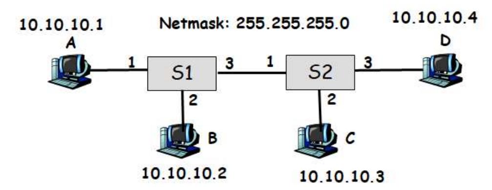
• (a) A sends an ARP request asking for the MAC address of B.

  Solution

  ARP Packet: <FF-FF-FF-FF-FF-FF, MAC_A, 0x0806><10.10.10.1, MAC_A, 10.10.10.2, 0-0-0-0-0-0>

  Broadcasts to all other ports on S1 (ports 2, 3), so B receives it. S2 also gets it from port 1 and floods to ports 2, 3 (so C and D receive it).

  S1 MAC Table: A → port 1 S2 MAC Table: A → port 1

• (b) B sends an ARP reply containing its MAC address.

  Solution

  ARP Packet: <MAC_A, MAC_B, 0x0806><10.10.10.2, MAC_B, 10.10.10.1, MAC_A>

  This is unicast (B knows A’s MAC), so only A receives it.

  S1 MAC Table:

  Host	Interface
  A	1
  B	2

  S2 MAC Table: A → port 1 (unchanged, this packet doesn’t go through S2)

• (c) A sends an IP packet to B.

  Solution

  IP Packet: <MAC_B, MAC_A, 0x0800><10.10.10.1, 10.10.10.2>

  Unicast from A to B (A now knows B’s MAC). No changes in tables since both MAC entries already exist.

  S1 MAC Table:

  Host	Interface
  A	1
  B	2

• (d) D sends an IP packet to A.

  Solution

  IP Packet: <MAC_A, MAC_D, 0x0800><10.10.10.4, 10.10.10.1>

  Unicast from D to A. S1 learns D’s MAC. S2 already knows where A is.

  S1 MAC Table:

  Host	Interface
  A	1
  B	2
  D	3

  S2 MAC Table: A → port 1; D → port 3

• (e) A sends an IP packet to 10.10.10.255.

  Solution

  IP Packet: <FF-FF-FF-FF-FF-FF, MAC_A, 0x0800><10.10.10.1, 10.10.10.255>

  Broadcast to all. S1 floods to all ports, S2 floods to all ports.

  S1 MAC Table:

  Host	Interface
  A	1
  B	2
  D	3

  S2 MAC Table: A → port 1; D → port 3; C → port 2

Problem 14: ARP Replies and Broadcast Handling in Switched LANs

Consider the following LAN consisting of two switches S1 and S2 connecting 4 hosts A, B, C and D. Assume a host H’s MAC address is MACH. The IP address of each host is shown in the Figure. Assume the netmask of each host is 255.255.255.0. Assume that the switch forwarding tables are empty to start with. For each of the following cases, show the forwarding tables of the switches and describe which hosts will receive the transmitted packet. For each IP packet show <Destination MAC, Source MAC, Type><Source IP, Destination IP>. For each ARP packet show <Destination MAC, Source MAC, Type><Source IP, Source MAC, Target IP, Target MAC>

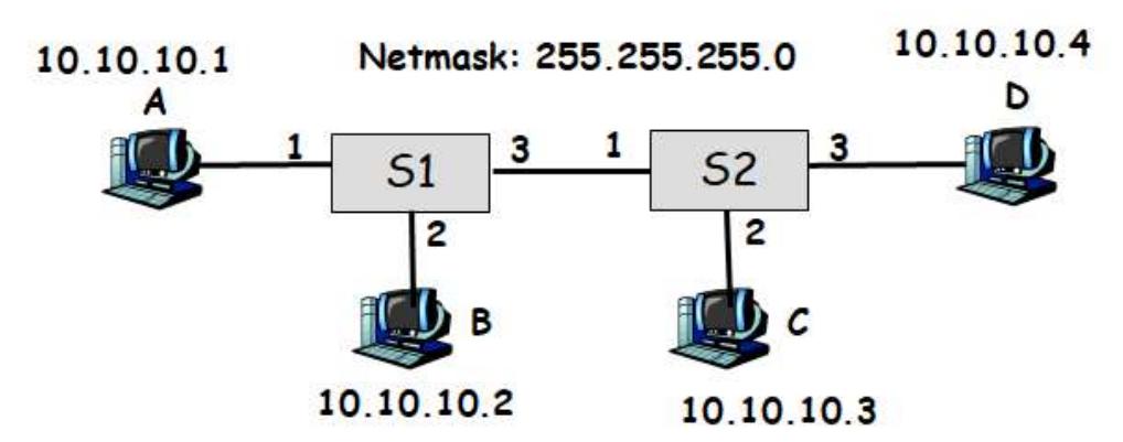
• (a) A sends an ARP request asking for the MAC address of D.

  Solution

  ARP Packet: <FF-FF-FF-FF-FF-FF, MAC_A, 0x0806><10.10.10.1, MAC_A, 10.10.10.4, 0-0-0-0-0-0>

  Broadcasts through S1 and S2. Both switches learn A’s MAC from this incoming packet.

  S1 MAC Table: A → port 1 S2 MAC Table: A → port 1

• (b) D sends an ARP reply containing its MAC address.

  Solution

  ARP Packet: <MAC_A, MAC_D, 0x0806><10.10.10.4, MAC_D, 10.10.10.1, MAC_A>

  Unicast reply from D back to A. Packet travels through S2 and S1, updating both tables.

  S1 MAC Table: A → port 1; D → port 3 S2 MAC Table: A → port 1; D → port 3

• (c) A sends an IP packet to D.

  Solution

  IP Packet: <MAC_D, MAC_A, 0x0800><10.10.10.1, 10.10.10.4>

  Unicast from A to D (A now knows D’s MAC). Both switches already have learned the MAC entries.

  S1 MAC Table: A → port 1; D → port 3 S2 MAC Table: A → port 1; D → port 3

• (d) B sends an IP packet to D.

  Solution

  IP Packet: <MAC_D, MAC_B, 0x0800><10.10.10.2, 10.10.10.4>

  Unicast from B to D. S1 learns B’s MAC. S2 already knows D.

  S1 MAC Table: A → port 1; D → port 3; B → port 2 S2 MAC Table: A → port 1; D → port 3

• (e) C sends an IP packet to 255.255.255.255.

  Solution

  IP Packet: <FF-FF-FF-FF-FF-FF, MAC_C, 0x0800><10.10.10.3, 10.10.10.255>

  Broadcast to all. S1 floods to all ports, S2 floods to all ports.

  S1 MAC Table: A → port 1; D → port 3; B → port 2 S2 MAC Table: A → port 1; D → port 3; C → port 2

Problem 15: Packet Encapsulation Across Router Boundaries

Consider the following network consisting of two links connected by a router. For each of the following cases show <Destination MAC, Source MAC, Type><Source IP, Destination IP> of a packet as it traverses from the source to the destination.

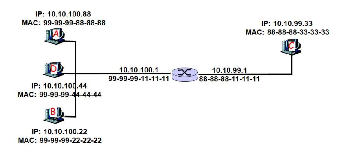
• (a) A sends a packet to B

  Solution

  A and B are on the same network (10.10.100.0/24).

  First, A sends ARP to find B’s MAC: <FF-FF-FF-FF-FF-FF, MAC_A, 0x0806><10.10.100.88, MAC_A, 10.10.100.22, 0-0-0-0-0-0>

  B responds: <MAC_A, MAC_B, 0x0806><10.10.100.22, MAC_B, 10.10.100.88, MAC_A>

  A sends the IP packet directly (no router needed): <MAC_B, MAC_A, 0x0800><10.10.100.88, 10.10.100.22>

• (b) C sends a packet to B

  Solution

  C is on 10.10.99.0/24, B is on 10.10.100.0/24 (different subnets). C must use the router.

  First, C sends ARP request to find the router (it broadcasts looking for a router on its subnet): <FF-FF-FF-FF-FF-FF, MAC_C, 0x0806><10.10.99.33, MAC_C, 10.10.100.22, 0-0-0-0-0-0>

  Router replies: <MAC_C, MAC_Router, 0x0806><10.10.99.1, MAC_Router, 10.10.99.33, MAC_C>

  C sends packet to router: <MAC_Router, MAC_C, 0x0800><10.10.99.33, 10.10.100.22>

  Router forwards to B’s link. Router sends ARP to find B’s MAC: <FF-FF-FF-FF-FF-FF, MAC_Router, 0x0806><10.10.100.1, MAC_Router, 10.10.100.22, 0-0-0-0-0-0>

  B responds: <MAC_Router, MAC_B, 0x0806><10.10.100.22, MAC_B, 10.10.100.1, MAC_Router>

  Router sends to B with rewritten MAC header: <MAC_B, MAC_Router, 0x0800><10.10.99.33, 10.10.100.22>

  Note: The IP addresses remain the same throughout. Only the MAC addresses change at each hop.

Problem 16: Address Resolution Protocol Overview

What’s the Address Resolution Protocol (ARP) and what is it used for. Does ARP run over the link layer or on top of IPv4? Briefly explain.

Solution

ARP runs on top of the link layer and discovers MAC addresses when you only know an IP address.

Problem 17: Internet Control Message Protocol Overview

What’s the Internet Control Message Protocol (ICMP) and what is it used for. Does ICMP run over the link layer or on top of IPv4? Briefly explain.

Solution

ICMP runs on top of IPv4 and is used as an error reporting when a host is not able to be reached. It can also run diagnostics if a host is alive via pings.

Problem 18: IPv4 Fragmentation Single Link

Suppose that a transport layer packet of size 2000 bytes is passed to IPv4 for delivery across one link, e.g., source and the destination hosts are on the same link. Assume that the MTU of the link is 500 bytes. Define the MTU of a link to be the maximum payload size of a link layer frame, i.e., maximum size of an IP packet that can fit into a Link Layer frame. Also, recall that the IP header size is 20 bytes. Schematically show the packets that are delivered to the network layer at the destination host by filling out the following table. Suppose the original IPv4 datagram is stamped with id number 100.

id	IPv4 length	IPv4 offset	IPv4 fragmentation flag

Solution

Each payload can be 500 - 20 = 480 bytes, so divide 2000 bytes into 480 byte pieces (plus 20 byte header):

id	IPv4 length	IPv4 offset	IPv4 fragmentation flag
100	500	0	1
100	500	480	1
100	500	960	1
100	500	1440	1
100	100	1920	0

Problem 19: IPv4 Fragmentation Multi-Link Path

Suppose that a transport layer packet of size 2048 bytes is passed to IPv4 for delivery across two links of the Internet (i.e., from the source host to a router to the destination host). The first link has an MTU of 1024 bytes; the second link has an MTU of 512 bytes. Define the MTU of a link to be the maximum payload size of a link layer frame, i.e., maximum size of an IP packet that can fit into a Link Layer frame. Also, recall that the IP header size is 20 bytes. Schematically show the packets that are delivered to the network layer at the destination host by filling out the following table. Suppose the original IPv4 datagram is stamped with id number 422.

After first link (1024 MTU):

id	IPv4 length	IPv4 offset	IPv4 fragmentation flag

At destination (after all refragmentation through second link with 512 MTU):

id	IPv4 length	IPv4 offset	IPv4 fragmentation flag

Solution

First link: 1024 MTU (payload is 1004 bytes) Second link: 512 MTU (payload is 492 bytes)

At destination (after all refragmentation):

id	IPv4 length	IPv4 offset	IPv4 fragmentation flag
422	512	0	1
422	512	492	1
422	512	984	1
422	512	1476	1
422	512	1968	1
422	40	2008	0

Problem 20: IPv4 Fragmentation with Bottleneck Link

Consider the following network. MTU of the link between A and R1 is 1500 bytes. MTU of the link between R1 and R2 is 512 bytes. MTU of the link between R2 and B is 1500 bytes. Assume that the transport layer gives a packet of size 2000 bytes to IPv4 for delivery to B. Define the MTU of a link to be the maximum payload size of a link layer frame, i.e., maximum size of an IP packet that can fit into a Link Layer frame.

Also, recall that the IPv4 header size is 20 bytes. Schematically show the packets that are delivered to the network layer at the destination host by filling out the following table. Suppose the original IPv4 datagram is stamped with id number 200.

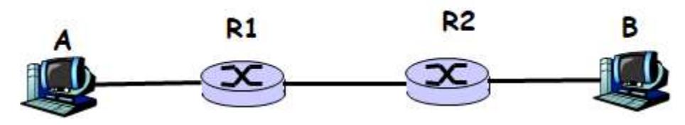
Schematically show the packets that are delivered to the network layer at the destination host (the following table has enough rows provided):

id	IPv4 length	IPv4 offset	IPv4 fragmentation flag

Solution

First link (1500 MTU): Payload is 1480 bytes Bottleneck link (512 MTU): Payload is 492 bytes Third link (1500 MTU): Payload is 1480 bytes

At destination (after all refragmentation):

id	IPv4 length	IPv4 offset	IPv4 fragmentation flag
200	512	0	1
200	512	492	1
200	512	984	1
200	512	1476	1
200	512	1968	0

Note: The fragments from the bottleneck link (second hop) fit easily into the larger payload of the third link, so they remain unchanged at the destination.

Problem 21: Network Address Translation Table Tracing

Consider the following network where network address translation (NAT) is being used. Assume that the Web browser running at host A sent a TCP connection request to the Web Server shown on the left side of the figure and the server replied back. During this conversation, the NAT router set up the NAT table shown on the figure. Show the source IP, source port, destination IP, destination port number of ALL packets that travel in the network from the time host A sends the TCP connection request, until the reply comes back from the server to host A.

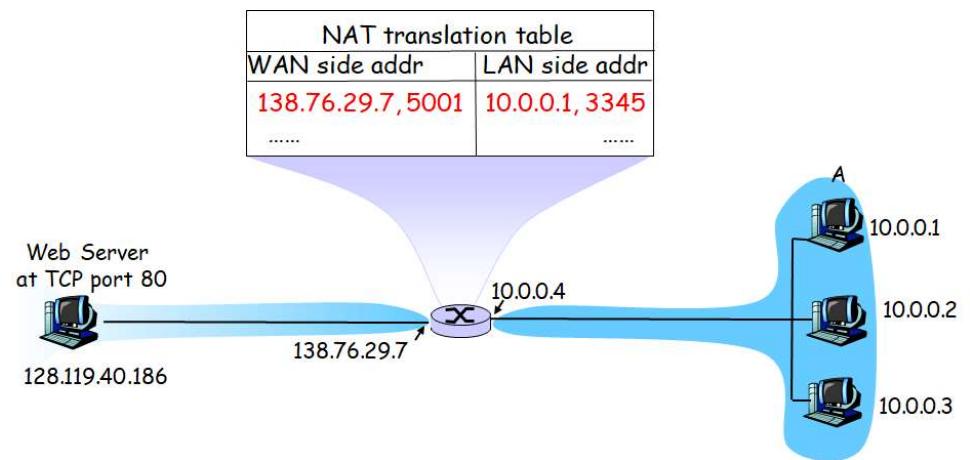
Packet	Source IP	Source PortNo	Dest IP	Dest PortNo
From A up to router
From router to Web Server
From Web Server to router
From router to A

Solution

Port 80 is the well-known HTTP port for web servers. Ports 2500, 3200, 4000 are ephemeral ports (assigned to the client).

The NAT router replaces the source IP and port in outgoing packets with the router’s external IP and a mapped port. On the return path, it reverses this mapping.

Packet	Source IP	Source Port	Dest IP	Dest Port
From A up to router	10.0.0.1	3345	128.119.40.186	80
From router to Web Server	138.76.29.7	5001	128.119.40.186	80
From Web Server to router	128.119.40.186	80	138.76.29.7	5001
From router to A	128.119.40.186	80	10.0.0.1	3345

Problem 22: Distance-Vector Routing Protocol

Consider the following network: Assume nodes run a distance-vector protocol to compute the shortest path to all destinations. Show the distance table at node A and derive the forwarding table.

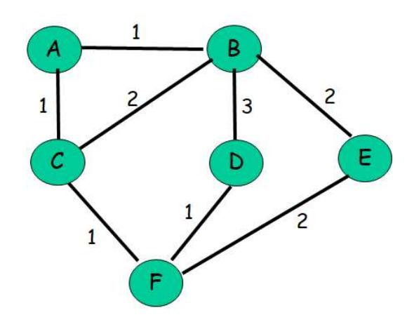
Destination	via B	via C
B
C
D
E
F

Destination	Next Hop
B
C
D
E
F

Solution

Distance Table at A:

Destination	via B	via C
B	1	3
C	3	1
D	4	3
E	3	4
F	4	2

Forwarding Table at A:

Destination	Next Hop
B	B
C	C
D	C
E	B
F	C

Explanation: For each destination, we choose the next hop (B or C) that gives us the minimum cost path.

Problem 23: Distance-Vector Routing Distance Table

Consider the following network: Assume nodes run a distance-vector protocol to compute the shortest path to all destinations. Show the distance table at node A and derive the forwarding table.

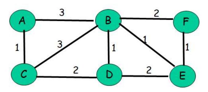
Destination	via B	via C
B
C
D
E
F

Destination	Next Hop
B
C
D
E
F

Problem 24: Dijkstra’s Shortest Path Algorithm

Consider the following network: With the indicated link costs, use Dijkstra’s shortest path algorithm to compute the shortest path from A to all network nodes. After computing the shortest paths from A to all other nodes, show the routing (forwarding) table constructed at A. Show your work clearly.

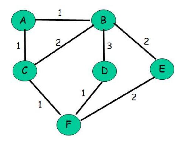
Problem 25: Dijkstra’s Algorithm from Different Source Node

Consider the following network: With the indicated link costs, use Dijkstra’s shortest path algorithm to compute the shortest path from F to all network nodes. After computing the shortest paths from F to all other nodes, show the routing (forwarding) table constructed at F. Show your work clearly.

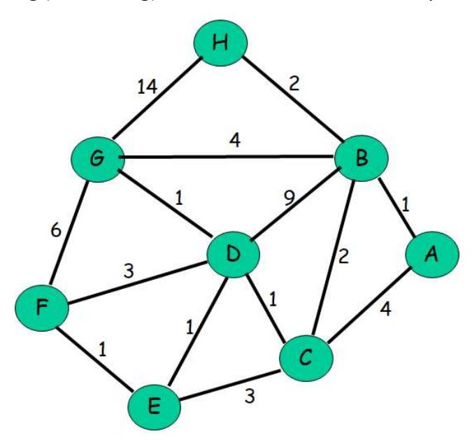
Problem 26: Multicast Routing Trees

Consider the network topology below.

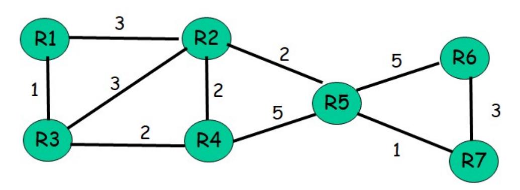
• (a) Assume router R1 is the source and reverse-path forwarding is used. Compute the resulting source-based multicast tree rooted at R1.
• (b) Assume center-based routing is used and router R4 is the core. Assume only routers R1, R2 and R6 have members that are part of the multicast group. Assuming that a router in the multicast group uses its least-cost path to node R4 to send join messages, draw the resulting center-based multicast routing tree. Is the resulting tree a minimum-cost Steiner tree. Justify your answer.