CSCI 381 Goldberg Lecture 3: Machine Language and Countability (Feb 2, 2026)

Administrative Updates

Course Setup Status

• Brightspace: Materials still being finalized (cloning from previous semester)
• All assignment dates are PLACEHOLDERS—IGNORE FOR NOW
• Official postings coming within next 1-2 days
• You will have sufficient time to complete assignments once dates are finalized
• Do NOT worry about Brightspace deadlines currently posted

Reading Assignment - TWO PAPERS REQUIRED (Critical)

Richard Karp’s Paper (1972)

• Full Title: “Reducibility Among Combinatorial Problems”
• Duration: Will spend 2-3 weeks analyzing this paper
• Significance: Demonstrates 20+ real-world problems are NP-hard/NP-complete
• Practical Applications: Despite being “pure theory,” has incredible practical real-world applications
• Why Important: Foundation for understanding computational complexity

Stephen Cook’s Paper (1971)

• Full Title: “The Complexity of Theorem-Proving Procedures”
• Duration: Will spend 1 day on this (foundation for Karp’s work)
• Significance: Introduced NP-completeness concept
• Age & Relevance: 54+ years old, still as relevant now as then

Important Context

• Both papers are extremely significant
• Cook’s paper (1971) established foundational concepts
• Karp’s paper (1972) extended to practical problems
• Together: Foundation of P vs NP problem

How to Get the Papers

Action Required:

1. Search online for author name + year + title
2. Download from Google Scholar, arXiv, or academic sources
3. Print physically OR save as PDF for class use
4. Have copies ready for next lecture (will reference extensively)

Course Materials Update

Brightspace Status

• Materials still being finalized (cloning previous semester)
• All assignment dates are PLACEHOLDERS - IGNORE FOR NOW
• Official postings coming within next 1-2 days

Ignore These For Now

• All Brightspace assignment deadlines
• Date fields posted in system
• Due dates in syllabus

When Finalized

• Professor will email official dates
• Links & materials will be updated
• You will have sufficient time to complete assignments

Attendance

• Text word “present” to register

Notes Distribution

• Emailed same day after class
• Check email later today for Lecture 3 notes

Next Steps

1. Search for and download both papers immediately
2. Have them ready for next lecture
3. Ignore all Brightspace assignment deadlines for now
4. Wait for official email with finalized dates

Lecture Content

Actual computation occurs at the lowest (hardware) of the machine. We call the language of that level, the machine language. In the case of the modern computer, the lowest level is binary based. We mentioned at the end of last class that the Natural numbers can be encoded using base 2 arithmetic (0/1) of finite length whereas arbitrary real numbers will require infinite length to describe/encode them due to the fractional/decimal portion (right of decimal point).

Martin Davis’s Key Insight: Arithmetic bases of ALL POSITIVE INTEGERS yield a computing device that is Turing Machine equivalent. Binary (base 2) is a convention, not a necessity.

Alternative Bases in Real Systems

• Base 3 (Trinary): Eastern European mainframes used base-3 because Shannon’s Information Complexity Theory (1948) showed the optimal base is e ≈ 2.87. Base 3 is closer to e than base 2, theoretically more efficient.
• Base 6: Developed for certain image processing systems; has special encoding properties
• Base 8 (Octal) & 16 (Hexadecimal): Used in assembly language systems
• Base 10: Used by abacus

Base 1 (Unary/Tally)

What is Base 1? A tally mark system where a number n is represented as n ones.

• Example: 4 = 1111, 5 = 11111
• Addition: Concatenation (“gluing” strings together)
• Example: 4 + 5 = 1111 + 11111 = 111111111 = 9
• Zero: Null string (empty)

Martin Davis proved base-1 can simulate all Turing machine computations.

Practical Speedup with Higher Bases

Research shows higher bases produce faster processing times (but not improved computability). Yet Analysis of Algorithms normalizes this away by dropping constants—all bases theoretically equivalent.

Why Not Real Numbers? Classic Turing Machine theory never considers real number arithmetic because:

1. No Successors: Real numbers lack a defined “next” number, making memory addressing impossible
2. Church-Turing Thesis: Computation only occurs over countable sets; real numbers are uncountable

Alonzo Church (1920s) American

Alan Turing (1930s) British

Church-Turing Thesis: Computation occurs (only) over Countable sets.

Countable Set is a set that is in a 1-1 correspondence with (a subset of the) Natural numbers.

A subsequent tab will demonstrate (based on Cantor’s writings) the manner with which one counts elements of a countable set can affect whether or not you can effectively accomplish the counting.

As opposed to the set of Real numbers, which is uncountable, proven by Georg Cantor (1880s) using a technique called diagonalization.

We will prove in the next tab that the real numbers are not countable. To do so, we will prove that the real numbers between 0 and 1, are not countable and since the complete set of real numbers is larger, they certainly are not countable. To further simplify our proof, we will describe the real numbers between 0 and 1 by binary expansion. Proof by contradiction. Assume that the real numbers are countable. Then, they can be sequentially ordered by a bijection with the Natural numbers.

The following Matrix stores every real number (under our current assumption that real numbers are countable). is the -th digit of the -th real number listed/counted in this matrix.

REAL#s i \DIGIT j	1	2	3	4	5	6		j
1	0	0	0	0	0	0		0
2	1	0	0	0	0	0		0
3	0	1	0	0	0	0		0
4	1	1	0	0	0	0		0
5	0	0	1	0	0	0		0
6	1	0	1	0	0	0		0
i

Now let us construct a (sort of) “random” real number and then check where on the above comprehensive listing of all real numbers can it be found. Consider all digits found on the diagonal of this matrix, .

We will construct a “new” real number .

Since Matrix has all possible real numbers, Rnew isn’t really all that “new” and must be found on this matrix.

So, which row is it?

Suppose Rnew can be found identically to the real number found on row of this matrix.

Then, for all , . This simply says that Rnew has to agree “bit by bit” with the -th row of matrix .

… … … … . .

Specifically, what value is ? The contradiction will be formed at one specific digit of this real number.

Since Rnew is found at row of the matrix , then for ; that is, . But that is NOT possible (!), since

According to the original definition of Rnew,

.

This contradicts the statement above that .

This contradiction implies that our original assumption that the set of Real numbers is countable

(which allowed to set up all the rows of this matrix in an order/sequential fashion)

is FALSE. Thus, the set of Real numbers is NOT countable.

The next tab gives other examples on how the same diagonalization argument can prove that other sets over the natural number are not countable.

Why is the quantitative aspect (“counting”) of set theory relevant to computing and computability?

This connection has to do with what we said earlier.

Any NATURAL number only requires a finite sequence of 0s and 1s

BUT, an arbitrary real number requires an infinite sequence of 0s and 1s.

COMPUTING devices by definition only have a finite memory storage (and even Turing’s infinite tape isn’t actually completely accessible during an effective computation.)

What about higher order bases? Base 3, 6, 8, 10, 16 and others

Base 3 arithmetic has a TRIT = Trinary digit has 0/1/2; whereas a BIT = Binary digit has 0/1

Computing mainframes in Eastern European countries used a Base 3 arithmetic and not a Base 2 arithmetic.

Shannon’s Information Complexity Theory (1948) and his notion of Entropy (information loss/gain) indicated that theoretically, a perfect representation of information is based on the arithmetic base “e” ~=2.87…. And since 3 is closer to “e” than 2 is, the Eastern European scientists argued that a base 3 computing device would be more efficient than a base 2 device.

Base 6 arithmetic has been developed for certain image processing systems.

Base 8 (octal) and Base 16 (hexadecimal) from assembly language systems.

Base 10 was used by the abacus.

According to Martin Davis, ALL POSITIVE INTEGERS can be used as the base for a Turing Machine equivalent computing device.

Martin Davis spends two chapters to prove this but mainly concentrates those chapters on proving a Base 1 arithmetic can yield a computing device that is Turing Machine equivalent. Logistically, how does such a machine perform arithmetic?

Martin Davis treats the memory values of a unary (base 1) machine as strings and not numbers per se.

(Note: This is for encoding purposes, not for numerical purposes. This is consistent with Turing’s view of mapping memory configurations.)

What does base 1 mean? Consider adding 4+5 = 9

, ,

Note: Here ”.” is an operator on strings called concatenation and simply “glues” the two string of four and five together, one after the other. According to this approach, zero is the null string.

HW. Despite the fact that the above analysis could show that ANY POSITIVE INTEGER base could enable a Turing Machine equivalent computing device, Base 1 will cause problems to Analysis of Algorithms tenets. (Not for submitting, but think about it; the answer will be available at end of semester.)

Since Martin Davis shows that any positive integer base will work for computing machines, is there any practical advantage to higher order bases? Research has shown that higher bases do in fact demonstrate faster processing time.

Sources: https://www.techopedia.com/why-not-ternary-computers/2/32427 for a fascinating discussion on this. Brian Hayes. (2001). “Third Base” in the Nov/Dec 2001 issue of American Scientist.

This consideration of higher order bases only affects complexity but does not affect computability.

Turing pursued the concept of effectiveness and not efficiency.

Recall that analysis of algorithms employs two simplifications for categorizing complexity

• 1. once the complexity of an algorithm has been identified, analysis of algorithms complexity will drop all lower order terms. For example, if time or space complexity was modeled by , then are the lower order (lower exponent) terms. This would leave Order of
  • “As the length of input () approaches infinity”, smaller order terms are negligible as compared to the main term of the complexity model formula.
• 2. having done that, analysis of algorithm complexity drops the constant in front of the highest order term, standardizing all such complexities as having a constant one in front of the highest order term. (normalization). The reason given is “speedup theorems”. Here, the complexity would then be stated as Order of , .

And, based on the laws of algorithms (as learned in Discrete Mathematics),

3. Changing bases only introduce an extra constant in the represented value. For example, consider a number represented separately in base with digits and again, in base with digits. Then, the difference in the number of digits the same value would require by base would (number of digits in base to represent ).

Putting this all together, although higher order numerical bases will provide faster processing times practically, the theoretical notion of complexity, as defined by analysis of algorithms, will ignore the “speedup factor” obtained because the constant factor in front of the highest order term will anyway be dropped according to analysis of algorithms complexity principles.

Which of the following data values can actually be stored as-is at the lowest level machine?

ITEM#	Data	Machine Level Direct Storage	Reason
1	$1.28	NO	There is no mechanism to store a ”$” directly at the machine level.
2	5	YES	Any nonnegative integer can trivially be stored at the machine level as a binary number.
3	-4	NO	There is no mechanism to store a ”-” directly at the machine level.
4	3.14	NO	There is no mechanism to store a ”.” directly at the machine level.
5	Steven	NO	The ability to store characters other than numbers at lowest level storage requires sophisticated encodings and not directly available.

The BOTTOM-LINE is that the lowest level of machine has simply a finite string (sequence) of 0s and 1s and NOTHING ELSE.

And, a single string/sequence of finite length of 0s and 1s can be encoded further as a SINGLE NONNEGATIVE INTEGER. This latter statement is a key observation used throughout computability theory.

Similarly, Genetic Algorithms (borrowing from Genetics) differentiates the underlying “machine level” (genotype) from the interpreted value level (phenotype). This itself stems (probably) from Greek philosophy which differentiated the “matter” (the underlying material of an object) from the “form” (an object’s characteristics and functionality). In data structure theory, this led to the notion of an “Abstract Data Type” (ADT).

Consider a Stack as an ADT. What conceptually characterizes a stack (its “form”)? Four operations: InitStack, StackEmpty, Push, Pop and a pointer to top element. As to how to implement a stack (its “matter”), two popular approaches are using a linked list or using an array, amongst others. Based on the conceptual understanding, there should be no way to access any data value on a stack that is below the top element. However, if you knew that the stack was implemented using an array (for example), then simple pointer/indexing arithmetic would give you access to elements below the top of the stack.

Previously, we differentiated between solvability and complexity. Solvable means that there exists an effective computation to solve your problem. Complexity is an efficiency consideration and is the analysis after determining solvability. The question arises how to define “easy” vs. hard in terms of complexity. Jack Edmonds (1960s) suggested that the distinction should be a purely mathematical one, polynomial vs exponential. This will be helpful in understanding Karp’s paper later in the semester.

Please search on the web for Richard Karp’s paper (1972) “Reducibility among combinatorial problems” and for Stephen Cook’s paper (1971) The complexity of theorem-proving procedures. Download/print these papers. I will be placing links on Brightspace within the week. We will need these paper for discussion during a number of forthcoming lectures.

Uncountability

Matrix-Based Representation: A Powerful Reinterpretation

Key Insight (Turing’s Perspective): The proof doesn’t depend on interpreting the matrix as real numbers. It depends only on the configuration of 0s and 1s in memory. Different interpretations of the same matrix produce different uncountability proofs.

Boolean Predicates

Definition: A Total Function mapping Natural numbers → {0,1}, where 0 = False, 1 = True.

(Note: Karp will later narrow this to require Boolean inputs as well.)

Why It’s Uncountable: A Boolean predicate is a row of 0s and 1s—exactly like matrix R rows. The identical diagonalization proof shows the set of all Boolean predicates is NOT countable.

Bitstrings

Definition: Finite sequences of 0s and 1s concatenated together (e.g., 0 1 0 1 1 0 1 ...).

Why It’s Uncountable: Same representation as matrix R rows. The identical diagonalization proof shows all bitstrings (arbitrary length) are NOT countable.

Critical Point: Whether you interpret the sequence as real number, Boolean predicate, or bitstring doesn’t matter for the proof—the configuration itself creates uncountability.

Power Set of Natural Numbers

Definition: A set is a collection of elements. Represent subsets S of N = {0, 1, 2, 3, …} as binary sequences where position i contains 1 if i ∈ S, else 0.

Example: 1 0 1 0 1 1 0 ... represents S = {0, 2, 4, 5, …}

Why It’s Uncountable: Again a matrix R row. The identical diagonalization proof shows Power Set(N) is NOT countable.

Summary: One proof, multiple interpretations demonstrate uncountability of:

• Real numbers (0 < x < 1)
• Boolean predicates over N
• All bitstrings (arbitrary length)
• Power Set of N

Effective vs. Ineffective Counting

Cantor’s Key Insight: Even if a set is countable, you must use an effective counting procedure. An ineffective procedure prevents counting the entire set. “Just start counting” doesn’t always work—you must be strategic.

Consider the Natural numbers. They are the basis for counting.

Let us start counting:

Counting by successors is effective. Here, successor = next element is obtained simply by .

How can we count this set in an ineffective manner that will prevent us from counting all the elements of the set, even though it is countable? The Natural numbers can also be thought as the Union of the Even numbers and the Odd Numbers.

• Even:
• Odd:

Example: Counting Evens and Odds

Effective Procedure for Even Numbers:
Effective Procedure for Odd Numbers:

Individually: Both are EFFECTIVE ✅ (count their respective sets completely)

Combined (count all evens, then all odds): INEFFECTIVE ❌ → Infinite loop on evens, never reach odds!

Lesson: Individual countability ≠ combined countability with sequential approach. The enumeration strategy matters.

Example: Counting Lattice Points in 2D (Cantor’s Solution)

The Problem: Effectively count all integral points (x, y) where x, y ≥ 0.

Each row or column independently: Countable (one dimension)

Naive Approach (INEFFECTIVE):

• Count row by row (or column by column)
• Infinite rows prevent finishing the first row
• Result: Infinite loop, never advance

Cantor’s Solution (EFFECTIVE): Count by diagonal

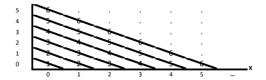
Diagonal approach ensures:

• Each diagonal has finite points only
• Each point reached in finite steps
• No infinite loops

Key Principle: Careless enumeration creates infinite loops even for countable sets. The counting procedure itself must be effective—smart strategy essential.