CSCI 381 Goldberg Lecture 4: Solvability, Complexity, and Computability (Feb 4, 2026)

Administrative Updates

Technical Updates - Brightspace Resolved

• Session limit issue FIXED - no more Part 2 session switching needed
• Can now run full 75-minute lectures in single Brightspace session
• Course schedule relatively stable for rest of semester

Assignments & Deadlines

Critical: Ignore Placeholder Dates

• Brightspace calendar currently has placeholder/outdated deadline dates
• ACTION: IGNORE all deadline dates shown in system
• What to do: Continue working on assignments at your own pace
• Real deadlines: Professor will email official dates when finalized
• Timeline: You WILL have sufficient time; no rush

Reading Materials - REQUIRED

If you haven’t already downloaded them:

Richard Karp’s Paper (1972)

• Title: “Reducibility Among Combinatorial Problems”
• Focus: Will spend multiple weeks analyzing this paper
• Significance: Demonstrates 20+ real-world problems are NP-complete
• Practical Use: Despite theoretical nature, has major practical applications

Stephen Cook’s Paper (1971)

• Title: “The Complexity of Theorem-Proving Procedures”
• Focus: One day of discussion (foundation for Karp’s work)
• Significance: Foundational NP-completeness concepts
• Note: 54+ years old, still highly relevant today

Action: Have printed or digital copies available for class.

Schedule Information

• Next Monday (Feb 10): Regular class session
• Following week: Some closures for presidential/federal holidays
• Dates TBA: Check calendar for exact holiday schedule before planning

Attendance

• Text word “present” to register attendance

Course Materials

• Notes emailed same day after class
• Check all email folders for professor messages

Lecture Content

Complexity vs. Solvability

While early computer theorists were less concerned with efficiency of time resources, analyzing different categories of algorithms requires us to consider time complexity. This notion will lead us to Karp’s famous 1972 paper and the fundamental problem of P vs NP.

We must distinguish two key concepts:

• Complexity — How much time is required to solve a problem
• Solvability — Whether a problem can be solved at all, independent of time (also called “decidability”)

A problem might be solvable, but require an unreasonably long time—even infinite time.

Important Preliminaries from Turing’s Model

Two critical points underpin our analysis:

1. Halting requirement: Infinite loops are not allowed. Turing’s definition requires that machines halt and produce output. The contents of memory after halting constitute the result.

2. Time vs. Memory: Although algorithms concern both resources, practical analysis focuses more on time since memory is typically abundant. However, complexity classes like incorporate both considerations.

Input Length and Time Complexity

Critical insight: time is based on the length of the input, not its value.

The relationship between a value and the number of bits needed to store it is exponential:

where is the minimum number of bits required to store value . Therefore, , which means .

This is crucial: An algorithm running in linear time with respect to input length is actually exponential in the magnitude of the value being processed.

Notation for Halting and Non-Halting

From Martin Davis, we use the notation:

• — Function halts when given input
• — Function does not halt when given input

Partially Computable vs. Computable Functions

Partially Computable (Recursively Enumerable):

If code exists that implements a function, that function is partially computable. The function may be partial—it does not need to halt for every input. It can loop indefinitely for some inputs.

Computable (Recursive):

If code is well-defined for all inputs (no infinite loops, every input produces output), the function is total and called computable. This is also called recursive in computation theory (unrelated to programming recursion).

---

Problem Categories: Decision vs. Optimization

Decision Problems

Decision problems return a boolean answer: Does a certain property or relationship hold true for the given input?

Example: “Is this number prime?”

Verification: Decision problems naturally support verification—once the algorithm provides an answer, users can check its correctness.

Optimization Problems

Optimization problems return a numerical answer: What is the best value (maximum or minimum) and how do we obtain it?

Examples: “Find the shortest path,” “Minimize cost,” “Maximize profit”

The Verification Challenge in Optimization

How can we verify that a proposed maximum is truly the global maximum across all possible inputs?

In calculus, we use the first derivative test: if , then might be optimal. But this is merely a necessary condition, not sufficient. Problems include:

1. First derivative test is necessary but not sufficient: If , then might be optimal, but the point could be a maximum, minimum, or saddle point.

2. Directionality: A critical point can be a maximum in one direction or a minimum in another direction—we must determine which using the second derivative test.

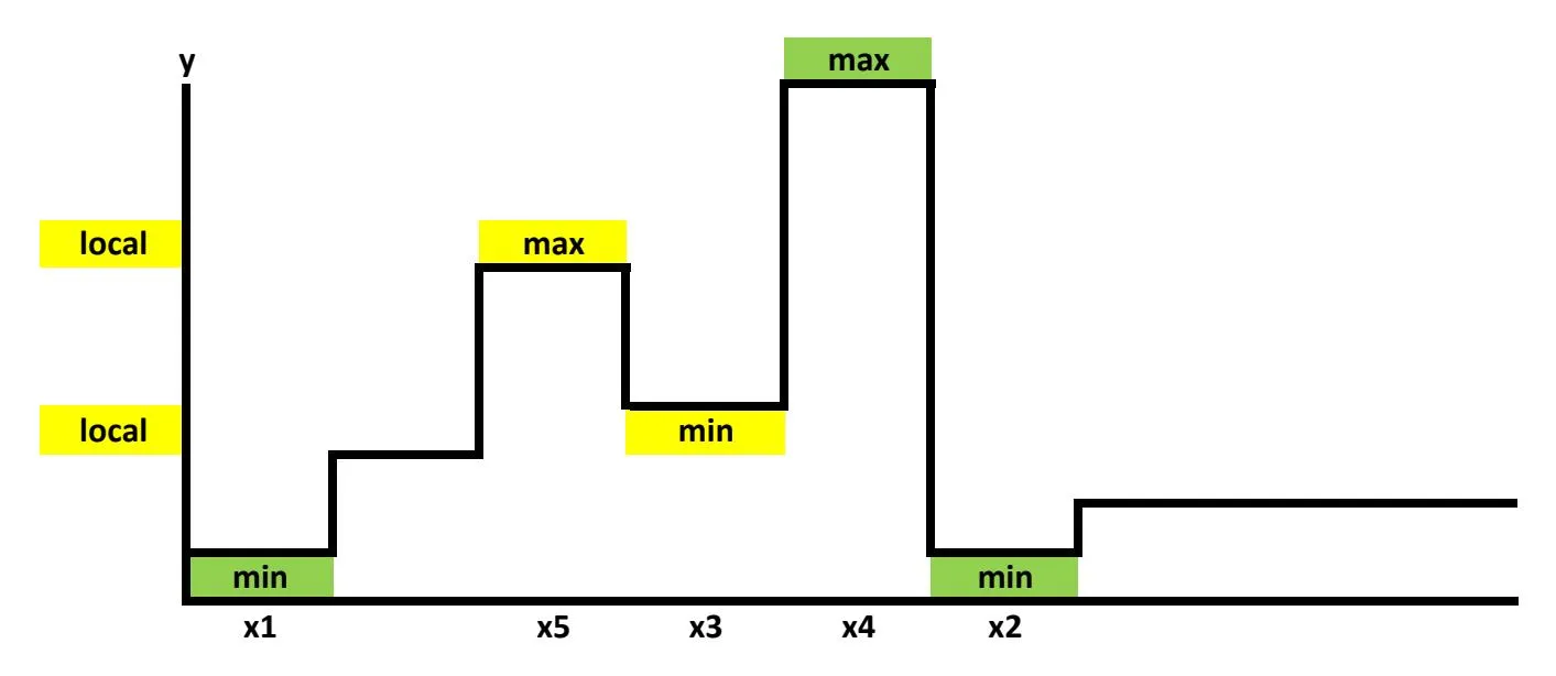
3. Saddle Points and Second Derivative Test: A critical point where can be neither a maximum nor a minimum. See this visualization for the function . A saddle point is called a hyperbolic paraboloid: in one direction (e.g., -direction) the curve is concave (∩), appearing like a maximum, but in the perpendicular direction (-direction) it is convex (∪), appearing like a minimum. At their intersection is the saddle point—neither a true maximum nor minimum.

   • The second derivative test helps distinguish:
     • If : local minimum
     • If : local maximum
     • If : possibly a saddle point

Global vs. Local Optimization

The second derivative test helps: the sign of indicates whether a point is a maximum, saddle point, or minimum.

However, from a computer science perspective, this is insufficient. While the second derivative identifies local optima, computer scientists seek the global optimum—the best solution across the entire domain—not just local improvement.

Exhaustive Search: The Brute-Force Approach

One way to find the global optimum: test every possible value in your domain (exhaustive search or brute-force). This is solvable but computationally expensive, requiring enormous time.

Karp’s Transformation Technique

Richard Karp addressed this verification problem by transforming optimization into decision:

1. Introduce a threshold parameter
2. Ask: “Is there a solution ≥ (or ≤ )?”
3. Now the optimization problem becomes a decision problem, which has natural verification

---

The Polynomial vs. Exponential Distinction

Objective Standards for Computation Time

A fundamental question: How do we distinguish between reasonable and unreasonable computation time?

Jack Edmonds’ Heuristic

Jack Edmonds proposed the standard. He was analyzing the Simplex algorithm for solving linear programming (LP) problems—systems of linear equations subject to constraints.

The Simplex algorithm works by:

1. Representing constraints as a convex polyhedron in solution space
2. Searching by jumping between corner points (endpoints) of the polyhedron
3. Making intelligent decisions about when to leave each corner point

A linear programming problem is a system of linear equations (where variables appear only to the first power, not squared or higher) subject to numerical constraints on variables. Edmonds was analyzing Danzig’s Simplex algorithm, which:

1. Encodes constraints as a convex polyhedron in solution space (a geometric shape with flat faces and corner points)
2. Searches by intelligently jumping from one endpoint (corner point) to the next
3. Makes optimal decisions about when to leave each corner

Edmonds conjectured that Simplex visits only a polynomial number of corners. If it visited exponentially many, the computation would be unreasonably slow.

Edmonds’ Distinction: Polynomial vs. Exponential

• Polynomial time: Essentially, a fixed number of nested loops. Reasonable.
• Exponential time: Exhaustive search trying every possible combination. Unreasonable (though still solvable, just very slowly).

Note: This is worst-case analysis. Better algorithms can sometimes prune the search space and achieve better bounds.

Karp’s P=NP Problem (1972)

Richard Karp adopted Edmonds’ distinction in his landmark paper, formulating P=NP in terms of polynomial time:

• P = Problems solvable in polynomial time (deterministic)
• NP = Problems verifiable in polynomial time (nondeterministic)

The question: Are these classes equal?

---

Deterministic vs. Nondeterministic Algorithms

Total Functions (Deterministic Models)

A total function maps inputs to outputs such that:

1. Every input has exactly one output (the “pencil test” from calculus)
2. There are no undefined inputs

Deterministic algorithms implement total functions:

• The program halts for every input
• At each step, exactly one next action is defined (no ambiguity)

Nondeterministic Algorithms (Stephen Cook & Theoretical Foundations)

Nondeterminism relaxes condition 2:

• The program still halts and produces output for every input
• At some point, instead of computing the next step deterministically, the program can make a nondeterministic choice guided by a Boolean predicate

Key Theoretical Foundation: According to work by Dijkstra (building on Floyd), deterministic and nondeterministic computation can be understood within standard programming frameworks. For instance, you could augment Java to create non-deterministic Java (njava), which would be identical to regular Java except for one additional command:

Choose a value for x from a set of values x1, x2, ..., xn
  such that some Boolean predicate p(xi) is true

This single command is the only addition needed to implement nondeterminism. All other Java features remain identical: loops, methods, classes, object-oriented programming, inheritance, recursion—the entire toolset.

Key clarification: Nondeterministic choices are not implemented as:

• A switch/case statement or cascading if-then-else (these are deterministic control flow)
• Random choice (unpredictable)

Rather, nondeterminism assumes the programmer provides the complete set of valid possibilities (satisfying the Boolean predicate), and the theoretical machine has the capability to instantly make the correct choice among them.

Simulating Nondeterminism Deterministically

Any nondeterministic computation can be simulated deterministically by trying all possible choices in a worst-case scenario. Whichever path leads to the correct solution is taken. From a solvability perspective, nondeterministic and deterministic machines solve exactly the same set of problems.

The difference lies in time: How long does it take to make the perfect choice?

The Time Distinction

Incorporating Edmonds’ heuristic:

• Polynomial time nondeterminism = Reasonable
• Exponential time nondeterminism = Unreasonable (but still solvable)

In Karp’s P=NP problem, “P” and “NP” both refer to polynomial time.

---

Approximation Approaches: Heuristics and Probabilistic Programming

Probabilistic and Randomized Methods

Rather than relying on the computer’s perfect foresight, an alternative is probabilistic programming: the algorithm makes “intelligent guesses” using random or statistical methods.

These approaches do not guarantee optimal solutions—only approximate ones.

Example: Genetic algorithms use random number generation and cannot guarantee perfect solutions, only approximate ones.

Heuristics are problem-solving techniques that provide approximate (not exact) solutions.

The Greedy Approach

A specific heuristic worth highlighting: the greedy approach states that at each decision point, choose the option offering the most immediate value, without considering future consequences.

Important caveat: Students often believe greedy always produces optimal solutions because textbooks present only cases where it succeeds. In reality, greedy is not guaranteed to be optimal.

---

Complexity Classes: C-Hard and C-Complete

For any complexity class :

• -hard: A problem at least as hard as any problem in (possibly harder)
• -complete: A problem that is -hard and whose solution can be verified within time complexity

For Karp’s work, (polynomial time algorithms).

Karp’s Strategy for Optimization Problems

Karp wanted to study complete problems whose solutions are easy to verify, yet many interesting problems are fundamentally optimization problems.

His solution: Transform optimization into decision by introducing a threshold and asking, “Is there a solution ≥ (or ≤ , as needed)?” This converts the optimization problem into a decision problem that can be verified in polynomial time.

One specific heuristic that deserves mention is the Greedy Approach, which states that when a decision should be made, whichever choice offers the most value right now is chosen, without considering what this choice will cause in the future. The importance for mentioning this is that students often mistakenly believe it always works.

---

Non-Determinism

The Concept of a Snapshot

To understand nondeterminism, we first need to define what Martin Davis calls a snapshot:

A snapshot captures the complete state of computation at any moment: which instruction is about to execute, and the values of all variables.

Deterministic Algorithms Revisited

Deterministic algorithms have a crucial property: given any snapshot, there is exactly one possible next instruction to execute. The decision is:

• Completely determined (decided ahead of time by the programmer’s design)
• Well-defined (no ambiguity)
• Based solely on the current snapshot (current variable values and position)

Additional requirements (from computation theory):

• Every input must eventually produce an output (no infinite loops)
• The program always halts

Note: The CPU’s Control Unit (along with the ALU - Arithmetic Logical Unit) is responsible for determining which instruction executes next based on the current state.

Nondeterministic Algorithms: Multiple Choices

Nondeterministic algorithms relax the determinism constraint:

Given a snapshot, it is not uniquely determined which instruction executes next. Instead, multiple valid choices may exist at that point in the code.

What Can Be Nondeterministic?

Nondeterministic choices affect two aspects of a snapshot:

1. Next instruction: More than one instruction might be valid to execute at this point (control flow nondeterminism)
2. Variable values: The values of variables in memory might have multiple valid options in “parallel universes” (data nondeterminism)—the same point in code could assign different values to the same variable

Critical Assumptions for Nondeterminism

For the nondeterministic model to be meaningful, certain assumptions must hold:

1. Garbage In, Garbage Out: Nondeterminism cannot fix programmer errors. If the Boolean predicate is incorrect or the set of values to choose from is incomplete, the machine won’t “magically” make it right. The choices offered must be correct from the outset.

2. Correctness of Choice: The machine always selects the correct choice from the offered possibilities. This is a theoretical assumption—the machine has perfect knowledge of which choice leads to the solution.

3. Turing’s Insight: Despite this seemingly magical assumption, Turing realized nondeterminism is not necessary for computational power. Any nondeterministic computation can be simulated deterministically by a brute-force exhaustive search trying all possibilities. Using parallel threads (each exploring one possibility), whichever thread reaches a solution first announces it. Turing himself simulated this using multiple tapes (sequentially), though parallelism is more efficient.

The Time Cost of Nondeterminism

The key issue with the nondeterministic “choose” command is its cost in time:

• In theory, the nondeterministic command executes in constant time
• The simulation of nondeterminism deterministically (trying all possibilities exhaustively) could take exponential time in the worst case

This time distinction is crucial to the P vs. NP problem:

• Polynomial-time nondeterminism is considered reasonable
• Exponential-time nondeterminism is considered unreasonable (though still solvable)

Solvability vs. Complexity: From a solvability perspective, nondeterministic and deterministic machines solve exactly the same set of problems. The difference is purely about time efficiency, not computational power.

---

Further exploration of nondeterminism and its applications to P vs. NP will continue in the next lecture.