Homework 1 - Modeling and Gradient Descent

This homework reviews general ideas about modeling, introduces the concept of gradient descent, and explores its practical application. The problems are color-coded by difficulty: green indicates easy problems, yellow indicates intermediate problems, and red indicates difficult problems.

Problem 1: Fundamentals of Modeling

(a) What is a model?

Solution

A model is a simplified representation of a real life object or process. We use these to mimic the behavior of more complex objects or processes. In essence, these are just approximations to reality.

(b) Give an example of a model (preferably one that was not discussed in class) and explain why this is a model.

Solution

An example of a model is the globe representing the Earth. The globe is a simplified representation of the Earth, as it shows the general shape and topological features of the Earth, but it does not capture all the details and complexities of the actual planet. It is a model because it allows us to understand and visualize the Earth’s geography without needing to see the entire planet in person.

(c) George Box stated that “All models are wrong …”. If all models are wrong, then why do we study models?

Solution

The reason we study models is because they can still be useful for understanding and predicting phenomena, even if they are not perfectly accurate. They can help us understand patterns and relationships in data so that we can make informed predictions and decisions based on those predictions.

(d) What is a mathematical model?

Solution

A mathematical model is a model where the inputs and the outputs are numerical. Essentially, it uses mathematical relationships to describe phenomena. For example, the equation $y = mx + b$ is a mathematical model that describes a linear relationship between $x$ and $y$.

(e) What are the two goals of modeling?

Solution

Prediction: Can the model tell us what will happen for a specific phenomenon?

Explanation: What causes the phenomenon and what drives the result?

In essence, we want to be able to predict what will happen and understand why it happens.

(f) Suppose there is some phenomenon that we wish to model. Do we usually know all of the inputs or drivers of this phenomenon?

Solution

No, we typically do not know all the inputs or drivers of a phenomenon - this is why we need to use models in the first place.

(g) In class, we stated that finding a function or a model can be difficult and that recent advancements in artificial intelligence, particularly machine learning, can help us. What is artificial intelligence?

Solution

Artificial Intelligence is when computers/programs emulate human thought:

• Having a program describe a picture
• Solving equations
• Recognizing objects/sounds/language

(h) In class, we stated that finding a function or a model can be difficult and that recent advancements in artificial intelligence, particularly machine learning, can help us. What is machine learning? (Use the most recent definition we discussed in class).

Solution

Machine Learning is the process of training a piece of software, called a model, to make useful predictions or to generate content from data.

(i) Read the section called History on this page: https://en.wikipedia.org/wiki/Machine_learning. What was one of the first machine learning models?

Solution

One of the first machine learning models was Arthur Samuel’s checkers-playing program, which learned to evaluate board positions and improve its performance over time.

(j) Read the section called History on this page: https://en.wikipedia.org/wiki/Machine_learning. How did Tom Mitchell define machine learning?

Solution

A computer program is said to learn from experience E with respect to some class of tasks T and performance measure P if its performance at tasks in T, as measured by P, improves with experience E.

(k) Read the section called History on this page: https://en.wikipedia.org/wiki/Machine_learning. True or False? The inspiration for neural networks comes from algorithms that mirrors the human brain/thought process.

Solution

True.

(l) True or False? All of artificial intelligence falls under machine learning.

Solution

False. Artificial intelligence is a broader field, inside of which machine learning is a part of.

(m) True or False? All of machine learning falls under artificial intelligence.

Solution

True.

Problem 2: The Need for Gradient Descent

(a) Suppose we have a bunch of data points $(x_1, y_1), (x_2, y_2), \ldots (x_n, y_n),$ and we wish to use a linear model to predict the value of $y$. What parameters (or values) are we looking to find?

Solution

We are looking to find the coefficients of the linear model, which typically include the slope and the intercept. In a simple linear regression model, we would be looking to find the values of $m$ (the slope) and $b$ (the intercept) in the equation $y = mx + b$.

(b) In order to find these parameters, we have to define a cost function. How many dimensions would be required to graph the cost function?

Solution

The cost function for a linear model with 2 parameters (slope and intercept) would require 3 dimensions to graph. This is because the cost function is $C(m, b)$, which depends on two variables: $m$ (the slope) and $b$ (the intercept). To visualize this relationship, we need one axis for $m$, one axis for $b$, and a third axis for the cost value $C(m, b)$ itself.

(c) Once we have our cost function, what exactly are we looking to do with this function? What is our primary objective?

Solution

The goal is to minimize the cost function, which means finding the parameter values that result in the lowest cost.

(d) Explain how a machine can use the cost function to learn better values for our parameters. A full answer would outline the algorithm being used for the computer/machine to learn.

Solution

A machine can use the cost function to learn better values for our parameters through an optimization algorithm called gradient descent. The algorithm works as follows:

1. Initialize parameters: Start with $m=0$ and $b=0$ (or some random values).
2. Calculate the cost $C$ for this $m$ and $b$ using the cost function.
3. Compute the partial derivatives of the cost function with respect to $m$ and $b$ to find the gradients.
4. Define $\alpha$ as the learning rate. It will be a small positive number (e.g., 0.01).
5. Update the parameters as follows:
   • $m_{new} = m_{old} - \alpha \frac{\partial C}{\partial m}$
   • $b_{new} = b_{old} - \alpha \frac{\partial C}{\partial b}$
6. Repeat steps 2-5 until the cost function $C$ converges to a minimum or until a specified number of iterations is reached.

(e) Using your answer above, explain what it means when we say the machine is learning?

Solution

When we say the machine is learning, we mean that it is iteratively adjusting its parameters (in this case, $m$ and $b$) based on the cost function and the gradients. The machine is considered to be learning because it is improving its performance on the task (predicting $y$ from $x$) by minimizing the cost function, which tells us that it is getting better at making predictions.

(f) Now suppose we have a bunch of data points $(x_1, y_1), (x_2, y_2), \ldots (x_n, y_n),$ and we wish to use a quadratic model to predict the value of $y$. That is, we wish to find real numbers $a$, $b$, and $c$ such that $\hat{y_i} = a{x_i}^2 + b{x_i} + c.$ How many dimensions would be required to plot the cost function? Can we actually graph this function? If not, then is there a particular technique we can use to find the minimum of the cost function?

Solution

The cost function for a quadratic model with 3 parameters ($a$, $b$, and $c$) would require 4 dimensions to graph. Since we cannot visualize 4-dimensional graphs, we can’t “cheat” our way out of this by graphing the cost function. Instead, we can use gradient descent to find the minimum of the cost function, just like we did for the linear model. The algorithm would be similar, but we would need to compute the gradients with respect to 3 parameters instead of 2.

Problem 3: Gradient Descent with Large Learning Rate

In class, we performed the gradient descent algorithm on $f(x) = (x-5)^2$ by starting at $x=0$ and using the learning rate, $\alpha = 0.1$.

(a) This time, perform the first three iterations of gradient descent on $f(x) = (x-5)^2$ by starting at $x=0$ and using the learning rate, $\alpha = 4$. Describe what happens.

Solution

Step 1: Compute the derivative of $f(x)$:

$$f'(x) = 2(x - 5)$$

Starting at $x_{old} = 0$:

• $f'(x) = 2(x - 5)$
• At $x = 0$, $f'(0) = 2(0 - 5) = -10$
• Update $x$: $x_{new} = x_{old} - \alpha f'(x_{old}) = 0 - 4(-10) = 40$
• At $x = 40$, $f'(40) = 2(40 - 5) = 70$
• Update $x$: $x_{new} = 40 - 4(70) = -240$
• At $x = -240$, $f'(-240) = 2(-240 - 5) = -490$
• Update $x$: $x_{new} = -240 - 4(-490) = 1720$

After the first 3 iterations, we see that $x$ has diverged by a large amount from the minimum (which is at $x=5$). This happened because the learning rate $\alpha = 4$ is too large, causing the updates to overshoot the minimum and diverge instead of converging towards it.

Problem 4: One Dimensional Gradient Descent Practice

For all of the parts below, let $f(x) = x^4 + x^3 - 2x^2$.

(a) Sketch a graph of $f(x)$.

Solution

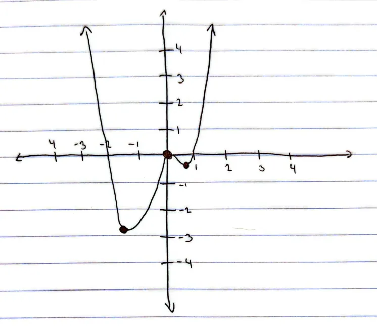
(b) Graphically, where is the global minimum of the function? If needed, round your answer to two decimal places.

Solution

Graphically, the global minimum of the function occurs at $\left(-1.44, -2.83\right)$ in the third quadrant of the graph.

To find the exact value, we compute the derivative and set it equal to $0$ to find the critical points ($x=-1.44$, $x=0$, or $x=0.693$), and then evaluate the function at those points.

(c) Now suppose we wish to find the global minimum by using gradient descent. Starting at $x=1$, compute what happens over the next three iterations. You may take the learning rate to be $\alpha = 0.1$.

Solution

Using:

$$x_{new} = x_{old} - \alpha f'(x_{old}), \qquad f'(x) = 4x^3+3x^2-4x$$

Starting at $x_{old} = 1$:

$$f'(x_{old}) = f'(1) = 4(1)^3 + 3(1)^2 - 4(1) = 4 + 3 - 4 = 3$$

Update $x$:

$$x_{new} = x_{old} - \alpha f'(x_{old}) = 1 - 0.1(3) = 0.7$$

At $x_{old} = 0.7$:

$$f'(0.7) = 4(0.7)^3 + 3(0.7)^2 - 4(0.7)$$ $$(0.7)^3 = 0.343, \quad (0.7)^2 = 0.49$$ $$f'(0.7) = 4(0.343) + 3(0.49) - 2.8$$ $$= 1.372 + 1.47 - 2.8 \approx 0.042$$

Update $x$:

$$x_{new} = 0.7 - 0.1(0.042) \approx 0.6958$$

At $x_{old} \approx 0.6958$:

$$f'(0.6958) = 4(0.6958)^3 + 3(0.6958)^2 - 4(0.6958)$$ $$(0.6958)^3 \approx 0.337, \quad (0.6958)^2 \approx 0.484$$ $$f'(0.6958) \approx 4(0.337) + 3(0.484) - 2.783$$ $$= 1.348 + 1.452 - 2.783 \approx 0.017$$

Update $x$:

$$x_{new} = 0.6958 - 0.1(0.017) \approx 0.6941$$

After 3 iterations, we have $x \approx 0.694$.

(d) If you had to guess, what value do you think our algorithm in Problem 4 Part (c) will converge to?

Solution

Based on the results of the first 3 iterations, it seems that the algorithm is converging towards a local minimum rather than the global minimum.

(e) Compute what happens after 500 iterations. You may use a calculator, Excel, or a programming language. Please explain what you did to get your answer.

Solution

def f(x: float) -> float:
    return x**4 + x**3 - 2 * x**2

def f_prime(x: float) -> float:
    return 4 * x**3 + 3 * x**2 - 4 * x

def gradient_descent(
    x_initial: float,
    alpha: float,
    iterations: int,
) -> float:
    x = x_initial
    for _ in range(iterations):
        x = x - alpha * f_prime(x)

    return x


x_initial = 1.0
alpha = 0.1
iterations = 500

x_final = gradient_descent(x_initial, alpha, iterations)

print(f"Result after {iterations} iterations, starting at x = {x_initial}:")
print(f"x_final = {x_final:.12f}")
print(f"f(x_final) = {f(x_final):.12f}")

Output:

Result after 500 iterations, starting at x = 1.0:
x_final = 0.693000468165
f(x_final) = -0.397046341000

I implemented the gradient descent algorithm in Python and ran it for 500 iterations with $x_{initial} = 1.0$ and learning rate $\alpha = 0.1$. The code defines 3 functions: $f(x)$, $f'(x)$ (the derivative), and the gradient descent function that iteratively updates $x$ using the update rule. After 500 iterations, the algorithm converged to approximately $x \approx 0.693$, at which point the function value is approximately $f(0.693) \approx -0.397$. This result lines up with our earlier approximations: starting from $x = 1$, the algorithm converges to a local minimum (not the global minimum, which occurs around $x \approx -1.44$). The algorithm was able to minimize the cost function from its initial position successfully, even though it converged to a local minimum instead of the global minimum.

(f) Now suppose we change our starting point to $x= -1$. Compute what happens over the next three iterations. You may take the learning rate to be $\alpha = 0.1$.

Solution

Using:

$$x_{new} = x_{old} - \alpha f'(x_{old}), \qquad f'(x) = 4x^3+3x^2-4x$$

Starting at $x_{old} = -1$:

$$f'(-1) = 4(-1)^3+3(-1)^2-4(-1) = -4+3+4 = 3$$

Update $x$:

$$x_{new} = -1 - 0.1(3) = -1.3$$

At $x_{old} = -1.3$,

$$f'(-1.3) = 4(-1.3)^3+3(-1.3)^2-4(-1.3)$$ $$(-1.3)^3 = -2.197,\quad (-1.3)^2 = 1.69$$ $$f'(-1.3) = 4(-2.197)+3(1.69)+5.2 = -8.788+5.07+5.2 = 1.482$$

Update $x$:

$$x_{new} = -1.3 - 0.1(1.482) = -1.4482$$

At $x_{old} = -1.4482$,

$$f'(-1.4482) = 4(-1.4482)^3+3(-1.4482)^2-4(-1.4482) \approx -0.06449$$

Update $x$:

$$x_{new} = -1.4482 - 0.1(-0.06449) \approx -1.44175$$

After 3 iterations (starting from $x=-1$), we have $x \approx -1.44175$.

(g) If you had to guess, what value do you think our algorithm in Problem 4 Part (f) will converge to?

Solution

It seems that the algorithm is converging towards the global minimum, which is approximately at $x = -1.44$.

(h) Do you think that in using gradient descent the starting point matters?

Solution

Yes, the starting point seems to act as a sort of initial guess for the algorithm and influences the path that the algorithm takes towards a minimum.