Homework 2 - Optimization and Kepler's Laws

This homework reviews optimization techniques including Newton’s method, explores the gradient descent proof, and applies proportional relationships to real-world astronomical data.

Problem 1: Reading and Analysis

(a) Read the article found here: https://www.quantamagazine.org/three-hundred-years-later-a-tool-from-isaac-newton-gets-an-update-20250324/. What date was this article published?

Solution

It was published on March 24, 2025.

(b) True or False? Most problems that involve finding an optimal solution boil down to minimizing a function.

Solution

True. The article states: “Mathematically, these problems get translated into a search for the minimum values of functions.”

(c) In the third paragraph, does the description of Newton’s method in optimization sound like any topic we discussed? If so, what topic? (Note that Newton’s method is sometimes called Newton-Raphson).

Solution

Yes, it sounds similar to gradient descent. Newton’s method works by using derivative information to iteratively find a better approximation of the minimum, similar to how gradient descent uses the slope to guide the search.

(d) In using Newton’s method in optimization, how many derivatives are required?

Solution

Two derivatives are required: the first derivative (slope) and the second derivative (the rate at which the slope is changing).

(e) What converges faster, Newton’s method or gradient descent? Note that the article states this answer and Wikipedia also has a nice visual: https://en.wikipedia.org/wiki/Newton%27s_method_in_optimization.

Solution

Newton’s method converges faster. It converges at a quadratic rate, while gradient descent converges at a linear rate. This means Newton’s method can identify the minimum value in fewer iterations.

(f) Given your answer above, why might someone opt to use gradient descent versus Newton’s method?

Solution

Newton’s method is more computationally expensive than gradient descent. Therefore, researchers prefer gradient descent for certain applications, such as training neural networks in machine learning, where the computational cost per iteration matters more.

(g) True or False? Ahmadi, Chaudhry and Zhang’s work “piggybacks” off previous work.

Solution

True. The article states: “Now Ahmadi, Chaudhry and Zhang have taken Nesterov’s result another step further.” Their work builds upon Yurii Nesterov’s 2021 breakthrough on approximating functions with cubic equations, extending it to work for arbitrarily many derivatives.

(h) What properties makes an equation easy to minimize?

Solution

Two properties make an equation easy to minimize: (1) The equation should be bowl-shaped or “convex,” with just one valley instead of many, so you don’t have to worry about mistaking a local valley for the global minimum. (2) If the equation can be written as a sum of squares, for example $5x^2 + 16x + 13 = (x+2)^2 + (2x+3)^2$.

(i) What did Ahmadi, Chaudhry and Zhang do to the Taylor expansion?

Solution

They added a “fudge factor” to the Taylor expansion using a technique called semidefinite programming. This modification made the Taylor approximation both convex and expressible as a sum of squares, without letting it drift too far from the original function it was meant to approximate.

(j) As of 2026, which technique is our best bet for optimization? Is it Newton’s, gradient descent or Ahmadi, Chaudhry and Zhang’s technique?

Solution

As of 2026, gradient descent is still the best bet for practical applications such as self-driving cars, machine learning algorithms, and air traffic control systems. While Ahmadi, Chaudhry and Zhang’s algorithm is theoretically faster, each iteration is still more computationally expensive than gradient descent.

(k) True or False? It is possible that Ahmadi, Chaudhry and Zhang’s technique can replace gradient descent in the future.

Solution

True. If computational technology becomes more efficient in the future, making each iteration of their algorithm less computationally expensive. Ahmadi hopes that in 10 to 20 years, their algorithm will also be faster in practice, not just in theory.

Problem 2: Proof of Gradient Descent Update Formula

Recall Mitchell’s definition of machine learning. A program is said to learn from experience $E$ with respect to some class of tasks $T$ and performance measure $P$ if its performance at tasks in $T$, as measured by $P$, improves with experience $E$.

(a) What is our goal in gradient descent? Specifically, if we are at $f(x_{old})$ then what can we say about $f(x_{new})$ in relation to $f(x_{old})$?

Solution

Our goal is to minimize the function. We want $f(x_{new})$ to be less than $f(x_{old})$, meaning we want to move to a point where the function value is smaller.

(b) Geometrically, what does it mean that $x_{new} = x_{old} + h$?

Solution

It means we are moving from the point $x_{old}$ by $h$ number of units. The variable $h$ indicates that we are either moving to the left (if $h < 0$) or to the right (if $h > 0$) on the number line.

(c) Suppose $f(x)$ is a differentiable function and we draw the tangent line to $f(x)$ at the point $(a, f(a) )$. What is the equation of this tangent line? Call the equation $L(x)$ where $L$ stands for linearization.

Solution

The equation of the tangent line is $L(x) = f(a) + f'(a)(x - a)$. This is the linearization of $f(x)$ at the point $a$.

(d) If $x$ is near $a$, then what can we say about $f(x)$ in relation to $L(x)$?

Solution

If $x$ is near $a$, then $f(x) \approx L(x)$. The linearization is a good approximation of the function near the point $a$.

(e) Let’s define $x := x_{old} + h = x_{new}$ and define $a := x_{old}$. What does your answer in part (d) become?

Solution

$$f(x) \approx L(x)$$ $$\Rightarrow f(x) \approx f(a) + f'(a)(x - a)$$ $$\Rightarrow f(x_{new}) \approx f(x_{old}) + f'(x_{old})(x_{old} + h - x_{old})$$ $$\Rightarrow f(x_{new}) \approx f(x_{old}) + h f'(x_{old})$$ $$\Rightarrow f(x_{new}) - f(x_{old}) \approx h f'(x_{old})$$

(f) Explain why $h f'(x_{old})$ is negative.

Solution

Since we need $f(x_{new}) < f(x_{old})$, then by subtracting $f(x_{old})$ from both sides, we get $f(x_{new}) - f(x_{old}) < 0$. Since $f(x_{new}) - f(x_{old}) \approx hf'(x_{old})$ and $f(x_{new}) - f(x_{old})$ is negative, $hf'(x_{old})$ must also be negative.

(g) Given your answer above, what does this imply about $h$?

Solution

For the inequality $hf'(x_{old}) < 0$ to hold, $h$ must always have the opposite sign of $f'(x_{old})$. For example, if both $h$ and $f'(x_{old})$ were negative, their product would be positive, violating our requirement that $hf'(x_{old}) < 0$.

(h) Why don’t we take $h = - f'(x_{old})$?

Solution

Taking $h = -f'(x_{old})$ directly can be an issue because the derivative $f'(x_{old})$ may be very large, resulting in excessively large jumps between consecutive function values. This can cause us to skip over the minimum entirely.

(i) What should we take $h$ to be?

Solution

We should take $h$ to be a small number: $h = -\alpha f'(x_{old})$ where $\alpha$ is a small positive scalar (like 0.01 or smaller).

(j) Substitute your answer above into $x_{new} = x_{old} + h$. What formula do we get?

Solution

Plugging $h = -\alpha f'(x_{old})$ into $x_{new} = x_{old} + h$ yields:

$$x_{new} = x_{old} - \alpha f'(x_{old})$$

(k) Intuitively, what does $\alpha$ represent?

Solution

$\alpha$ is the learning rate, which determines how big of a step we take at each iteration when updating $x$.

Problem 3: Mitchell’s Definition and Linear Models

Recall Mitchell’s definition of machine learning. A program is said to learn from experience $E$ with respect to some class of tasks $T$ and performance measure $P$ if its performance at tasks in $T$, as measured by $P$, improves with experience $E$.

Suppose we are interested in predicting a student’s score on a final exam.

For student $i$, let:

• $x_{i1}$ = hours spent studying (over the semester),
• $x_{i2}$ = number of class meetings attended,
• $x_{i3}$ = homework average (as a percent),
• $y_i$ = final exam score (from $0$ to $100$).

Assume we use the linear model

$$\hat{y}_i = b + m_1 x_{i1} + m_2 x_{i2} + m_3 x_{i3}$$

(a) What would the dataset, $\mathbb{D}$, look like?

Solution

The dataset $\mathbb{D}$ would contain all the tuples $(x_{i1}, x_{i2}, x_{i3}, y_i)_{i=1}^n$ for each of the $n$ students, where $x_{i1}$ is the hours they studied, $x_{i2}$ is the number of class meetings they attended, $x_{i3}$ is their homework average as a percent, and $y_i$ is their final exam score. In table form, the columns would represent each variable, and each row would represent one student’s data:

Hours Studied	Classes Attended	Homework Avg (%)	Exam Score
40	23	90	85
30	20	85	80
50	25	95	95
$\vdots$	$\vdots$	$\vdots$	$\vdots$

(b) In the context of Mitchell’s definition, what is $T$?

Solution

The task $T$ in Mitchell’s definition is the students’ hours studied, number of classes attended, and homework average.

(c) In the context of Mitchell’s definition, what is a good way to define $P$?

Solution

A good way to define the performance measure $P$ is to use a metric that quantifies how well the model’s predictions match the actual exam scores. For example, we could use the mean squared error (MSE) between the predicted scores $\hat{y}_i$ and the actual scores $y_i$:

$$\text{MSE} = \frac{1}{n} \sum_{i=1}^n ({y}_i - \hat{y}_i)^2$$

where $\hat{y}_i = b + m_1 x_{i1} + m_2 x_{i2} + m_3 x_{i3}$

(d) In the context of Mitchell’s definition, what is $E$?

Solution

The experience $E$ is all the data points $(x_{i1}, x_{i2}, x_{i3}, y_i)_{i=1}^n$ from the dataset $\mathbb{D}$ that we use to train the model.

(e) What happens in the training step? Try to be as detailed as possible.

Solution

We start by dividing $\mathbb{D}$ into three separate parts: a training set (80% of $\mathbb{D}$), a validation set (10% of $\mathbb{D}$), and a test set (10% of $\mathbb{D}$). Using the training set, we try different learning rates $\alpha_1, \alpha_2, \ldots, \alpha_t$. For each learning rate $\alpha_i$, we perform gradient descent to find the optimal parameters $b_i, m_{1i}, m_{2i}, m_{3i}$. For example, $\alpha_1$ yields $(b_1, m_{11}, m_{21}, m_{31})$, $\alpha_2$ yields $(b_2, m_{12}, m_{22}, m_{32})$, and so on until $\alpha_t$ yields $(b_t, m_{1t}, m_{2t}, m_{3t})$.

(f) What happens in the validation step?

Solution

In the validation step, we calculate the performance measure $P$ for every candidate model $(\alpha_i, b_i, m_{1i}, m_{2i}, m_{3i})_{i=1}^t$. We then select the parameters that yield the best performance, meaning the lowest MSE on the validation set.

(g) What happens in the test step?

Solution

In the test step, we use the best model we selected from the validation step and evaluate its performance on the test set, which contains data that the model has never seen before.

Problem 4: Kepler’s Laws of Planetary Motion

In the house pricing example discussed in class, we made the erroneous assumption that the house price was a linear function of square footage. During office hours, a student had asked “Does linear data actually appear in real life?” Allow us to now study a different phenomenon.

Definition: Proportional Relationship

Two quantities $x$ and $y$ are proportional if there exists a constant $k$ such that

$$y = kx \text{ for all } x \text{ and we write } y \propto x$$

which is read as ”$y$ is proportional to $x$”. The constant $k$ is called the constant of proportionality. Equivalently, whenever $x\neq 0$,

$$\frac{y}{x}=k \quad \text{(where again, $k$ is a constant).}$$

For instance, $y = 2x$, $y = 3x$, $y = 245.01x$ are all proportional relationships. How can we use this definition in modeling? Suppose we see the following data of the form $(x_i, y_i)$:

$$\mathbb{D} = \{ (1,3.1), (2,5.8), (3,8.85), (4,12.12) \}$$

and we want to find out if this data follows a proportional relationship. What we could do is take each value of $y$ and divide by $x$. If every quotient gives roughly the same constant $k$, then it is reasonable to build a model of the form $\hat{y_i} = kx_i$. Let’s investigate:

$x$	$y$	$k=\frac{y}{x}$
1	3.1	3.1
2	5.8	2.9
3	8.85	2.95
4	12.12	3.03

Since all of the quotients are near $3$, then it’s perhaps reasonable to say that $\hat{y_i} = 3x_{i}$. With this example in mind, let’s see the following application of proportionality which was discovered approximately 400 years ago.

(a) In astronomy, the orbital period refers to the amount of time it takes for a planet to complete one orbit around the Sun. For instance, the orbital period of Earth is about 365 days since it takes the Earth 365 days to move $360°$ around the Sun. Using the Internet, find out the orbital period for the following planets and fill out the chart. Please include your source by providing a link.

Solution

Planet	Orbital Period (measured in Days)
Mercury	88
Venus	225
Earth	365
Mars	687
Jupiter	4,333
Saturn	10,759
Uranus	30,687
Neptune	60,190

Source: https://spaceplace.nasa.gov/years-on-other-planets/en/

(b) Kepler’s First Law of Planetary Motion posits that each planet’s orbit about the Sun is an ellipse. Given an ellipse, consider the line segment which runs through the two foci and touches the perimeter of the ellipse. We call this line segment the major axis and half of the major axis is called the semi-major axis.

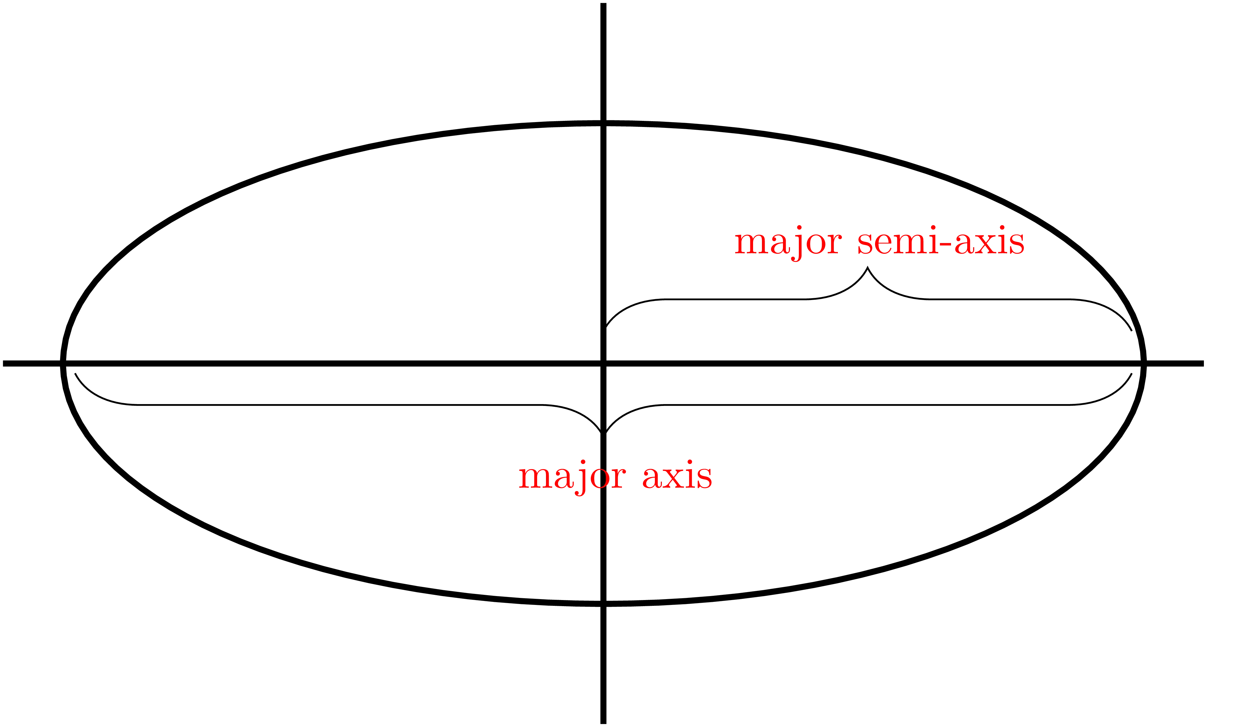
Using the Internet, find the length of the semi-major axis for each planet’s ellipse. Please include your source by providing a link.

Solution

Planet	Major Semi-Axis (measured in AU, Astronomical Units)
Mercury	0.387
Venus	0.723
Earth	1.0
Mars	1.524
Jupiter	5.204
Saturn	9.5826
Uranus	19.218
Neptune	30.110

Source: https://en.wikipedia.org/wiki/Semi-major_and_semi-minor_axes

(c) Suppose $x$ denotes the length of the major semi-axis while $y$ denotes the orbital period. Does it seem likely that $y \propto x$? If so then estimate the proportionality factor, $k$. Be sure to explain your answer.

Solution

$x$ (Semi-Major Axis)	$y$ (Orbital Period in days)	$k = y/x$
0.387	88	227.4
0.723	225	311.2
1.0	365	365.0
1.524	687	451.1
5.203	4,333	832.7
9.537	10,759	1,127.6
19.191	30,688	1,599.9
30.069	60,182	2,001.4

Based on the table above, $y \propto x$ does not hold because the ratios $k = y/x$ is changing by a large amount.

(d) Does it seem likely that $y^2 \propto x^3$? If so then estimate the proportionality factor, $k$. What does this imply?

Solution

$x^3$ (Semi-Major Axis Cubed)	$y^2$ (Orbital Period Squared in days²)	$k = y^2/x^3$
0.0579	7,744	133,780.9
0.3777	50,625	134,126.9
1.0	133,225	133,225.0
3.5398	471,969	133,298.1
140.7644	18,774,889	133,341.4
867.6277	115,755,081	133,438.8
7,070.3024	941,750,144	133,221.7
27,181.7117	3,621,873,124	133,309.1

Yes, according to the table it seems that $y^2 \propto x^3$ holds up well. The proportionality factor $k = y^2/x^3$ stays roughly constant at about 133,320. This means we can represent this relationship as $y^2 = 133,320 \cdot x^3$. Even though $y \propto x$ didn’t work, a hidden relationship was found by transforming the variables.