Homework 3 - Calculus, Perceptrons, and Neural Networks

This homework reviews calculus concepts, perceptron and sigmoid neuron fundamentals, and explores neural networks for digit recognition.

Problem 1: Crash Course Calculus Review

In this exercise, we will review some of the crash course calculus concepts that we discussed in lecture.

(a) Explain how the usual slope formula, $m = \frac{y_2 - y_1}{x_2 - x_1}$, can be used to develop the formula for the derivative.

Solution

If we have a function where we want to find the rate of change at a single point, then we want the slope of the tangent line at the point $(x, f(x))$. We can find a nearby point on the function, which we can call $(x + h, f(x + h))$. Using these two points, we can approximate the slope of the tangent line $m_T$ with the slope formula:

$$m_T \approx \frac{f(x + h) - f(x)}{x + h - x}$$

By combining like terms $x$ and $-x$ in the denominator, we get:

$$m_T \approx \frac{f(x + h) - f(x)}{h}$$

As we let $x + h$ get closer to $x$ as much as possible, or in other words, let $h$ approach 0, we obtain:

$$m_T = \lim_{h \to 0} \frac{f(x + h) - f(x)}{h}$$

which is the formula for the derivative.

(b) Let $f(x,y) = x^2 + y^2 - xy^2$. Sketch the graph of $f$. You may use a 3D graphing calculator such as https://www.desmos.com/3d.

Solution

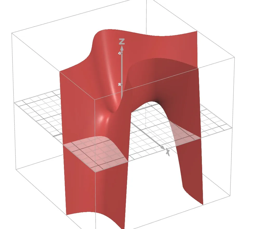
(c) Let $f(x,y) = x^2 + y^2 - xy^2$. Find $f_x(5,0)$.

Solution

We compute the partial derivative with respect to $x$:

$$f_x(x, y) = \frac{\partial f}{\partial x} = \frac{\partial}{\partial x} \left[x^2 + y^2 - xy^2\right] = 2x - y^2$$

Evaluating at the point $(5,0)$:

$$f_x(5, 0) = 2(5) - 0^2 = 10$$

(d) Geometrically, what does $f_x(5,0)$ represent?

Solution

It represents the slope of the tangent line in the $x$ direction to the surface $f(x, y) = x^2 + y^2 - xy^2$ at the point $(5,0)$. Since $f_x(5,0) = 10$, the surface is rising in the $x$ direction at the point $(5,0)$ with a slope of 10.

(e) Let $f(x,y) = x^2 + y^2 - xy^2$. Find $f_y(5,0)$.

Solution

We compute the partial derivative with respect to $y$:

$$f_y(x, y) = \frac{\partial f}{\partial y} = \frac{\partial}{\partial y} \left[x^2 + y^2 - xy^2\right] = 2y - 2xy$$

Evaluating at the point $(5,0)$:

$$f_y(5, 0) = 2(0) - 2(5)(0) = 0$$

(f) Geometrically, what does $f_y(5,0)$ represent?

Solution

It represents the slope of the tangent line in the $y$ direction to the surface $f(x, y) = x^2 + y^2 - xy^2$ at the point $(5,0)$. Since $f_y(5,0) = 0$, the surface remains flat in the $y$ direction at the point $(5,0)$ due to the slope being 0.

Problem 2: Two-Dimensional Gradient Descent

In this exercise, we will explore gradient descent a bit more. Consider the two-dimensional cost function below:

$$f(x, y) = (x - 3)^2 + (y - 2)^2$$

(a) Compute $\frac{\partial f}{\partial x}$.

Solution

$$\frac{\partial f}{\partial x} = \frac{\partial}{\partial x} \left[(x - 3)^2 + (y - 2)^2\right] = 2(x - 3)$$

(b) Compute $\frac{\partial f}{\partial y}$.

Solution

$$\frac{\partial f}{\partial y} = \frac{\partial}{\partial y} \left[(x - 3)^2 + (y - 2)^2\right] = 2(y - 2)$$

(c) Perform the next two iterations of gradient descent starting at $(x_0, y_0) = (0, 0)$ with a learning rate of $\alpha = 1$.

Solution

Iteration 1:

Evaluate the cost function and partial derivatives at $(0, 0)$:

$$f(0, 0) = (0 - 3)^2 + (0 - 2)^2 = 13$$ $$f_x(0, 0) = 2(0 - 3) = -6, \quad f_y(0, 0) = 2(0 - 2) = -4$$

Update using $\alpha = 1$:

$$x_{\text{new}} = x_{\text{old}} - \alpha f_x(x_{\text{old}}, y_{\text{old}}) = 0 - (1)(-6) = 6$$ $$y_{\text{new}} = y_{\text{old}} - \alpha f_y(x_{\text{old}}, y_{\text{old}}) = 0 - (1)(-4) = 4$$

Iteration 2:

Evaluate the cost function and partial derivatives at $(6, 4)$:

$$f(6, 4) = (6 - 3)^2 + (4 - 2)^2 = 13$$ $$f_x(6, 4) = 2(6 - 3) = 6, \quad f_y(6, 4) = 2(4 - 2) = 4$$

Update using $\alpha = 1$:

$$x_{\text{new}} = x_{\text{old}} - \alpha f_x(x_{\text{old}}, y_{\text{old}}) = 6 - (1)(6) = 0$$ $$y_{\text{new}} = y_{\text{old}} - \alpha f_y(x_{\text{old}}, y_{\text{old}}) = 4 - (1)(4) = 0$$

(d) Draw an analogy between minimizing a cost function in machine learning and tuning a guitar.

Solution

When guitar players tune their instruments and notice a string is out of tune, they gradually adjust the tuning peg by turning it tighter or looser until the pitch sounds correct. Minimizing a cost function in machine learning is analogous in the sense that the cost function measures how incorrect the model’s predictions are, and we use gradient descent to adjust parameters in the direction that reduces this error. In both cases, we iteratively make small adjustments based on the feedback we get, whether it’s the sound of the pitch or the value of the cost function, until we reach a desired state.

Problem 3: The Perceptron

In this question we will review the perceptron.

(a) Explain what is meant by the perceptron? A good answer would discuss what the inputs and outputs are.

Solution

The perceptron is a piecewise function that takes in several binary inputs and returns a binary output. The inputs $x_1, x_2, \ldots, x_n$ and the output $y$ are all equal to 0 or 1. Attached to the inputs are weights $w_1, w_2, \ldots, w_n \in \mathbb{R}$ that measure how much each respective input should affect the output. There is also a bias term $b \in \mathbb{R}$ that measures how easy it is for the perceptron to output a 1.

(b) In the perceptron, what function do we use to compute the output?

Solution

$$\text{Perceptron Output} := \begin{cases} 0 & \text{if } w_1 x_1 + w_2 x_2 + \cdots + w_n x_n + b \leq 0 \\ 1 & \text{if } w_1 x_1 + w_2 x_2 + \cdots + w_n x_n + b > 0 \end{cases}$$

(c) Consider the single layer perceptron below.

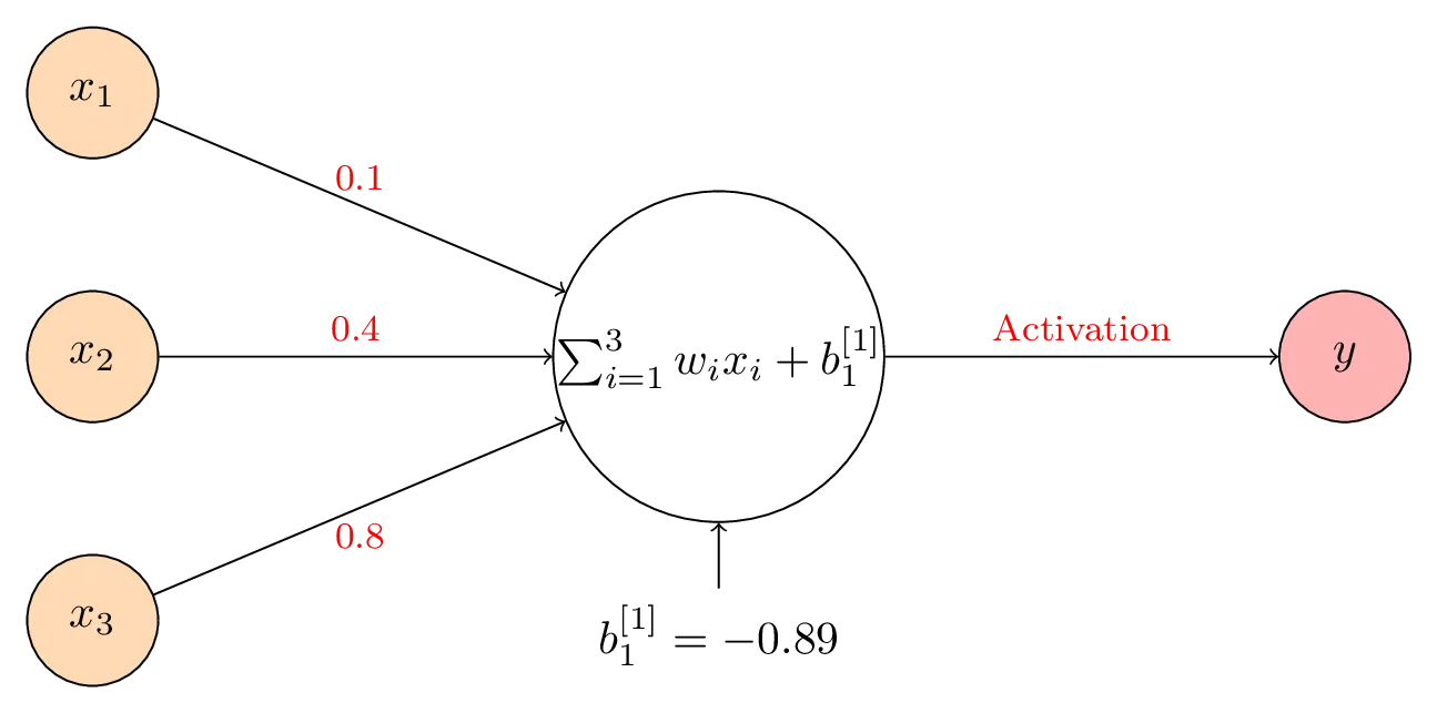
Suppose $x_1 = 1, x_2 = 0, x_3 = 1$. Also suppose that $b\_{1}^{[1]} = -0.89$. Compute the perceptron’s output. Hint: remember that a perceptron’s output is either 0 or 1.

Solution

We apply the perceptron function from part (b) and evaluate the weighted sum:

$$w_1 x_1 + w_2 x_2 + w_3 x_3 + b_1^{[1]} = (0.1)(1) + (0.4)(0) + (0.8)(1) - 0.89 = 0.01$$

Since the result $0.01 > 0$, the perceptron outputs $1$.

(d) In class, we stated that for the perceptron, small changes in the input can produce large changes in the output. Suppose we have the same perceptron as outlined above where $x_1 = 1, x_2 = 0, x_3 = 1$ and this time, $b\_{1}^{[1]} = -0.9$. What is the perceptron’s output now?

Solution

We apply the same function to get:

$$w_1 x_1 + w_2 x_2 + w_3 x_3 + b_1^{[1]} = (0.1)(1) + (0.4)(0) + (0.8)(1) - 0.9 = 0 \leq 0$$

Since the weighted sum equals 0, the perceptron outputs 0.

(e) In class, we stated that there were two fundamental restrictions with the perceptron. What are these restrictions/problems?

Solution

The first restriction is that the perceptron output is entirely binary (either 0 or 1) and very sensitive to small input changes. This means that a tiny adjustment to an input can result in a completely different output. The second restriction is that the perceptron, while a reasonable attempt to model how humans make decisions, is too limited to capture the full complexity of human decision-making. We can address this limitation by introducing hidden layers to make the model more sophisticated.

(f) Read the article found here: https://news.cornell.edu/stories/2019/09/professors-perceptron-paved-way-ai-60-years-too-soon. According to the article, what was one of the problems with Roseblatt’s perceptron?

Solution

One issue with Rosenblatt’s perceptron was that it had only a single layer, which made it insufficient for more complex tasks like computer vision and language processing.

Problem 4: The Sigmoid Neuron

In the previous question we identified the shortcomings of the perceptron. We now aim to review its upgrade — the sigmoid neuron.

(a) How is the sigmoid neuron different from the perceptron? Phrased differently, why is the sigmoid neuron more flexible than the perceptron?

Solution

The sigmoid neuron differs from the perceptron because it allows the inputs $x_1, x_2, \ldots, x_n$ to be any real number and allows the output $y$ to be any real number between 0 and 1. This makes it more flexible than the perceptron since it removes the constraint that inputs and outputs must be strictly binary. Rather than using a piecewise step function like the perceptron, the sigmoid neuron has a smooth activation function:

$$\sigma(z) = \frac{1}{1 + e^{-z}}$$

where $z = w_1 x_1 + w_2 x_2 + \cdots + w_n x_n + b$.

(b) Allow us to reconsider the neural network above:

Suppose the activation function is now the sigmoid function. Compute the output of the sigmoid neuron when $x_1 = 1, x_2 = 0, x_3 = 1$. (This is the same input as before in Problem 3 part (c)).

Solution

First, we calculate the weighted sum:

$$z = w_1 x_1 + w_2 x_2 + w_3 x_3 + b_1^{[1]} = (0.1)(1) + (0.4)(0) + (0.8)(1) - 0.89 = 0.01$$

Next, we apply the sigmoid function:

$$\sigma(0.01) = \frac{1}{1 + e^{-0.01}} \approx 0.5025$$

(c) Allow us to now show that a small change in the weights/bias produces small changes in the output. Suppose we have the same sigmoid neuron as outlined above where $x_1 = 1, x_2 = 0, x_3 = 1$ and this time, $b\_{1}^{[1]} = -0.9$. What is the sigmoid neuron’s output now?

Solution

We compute the weighted sum with the new bias:

$$z = w_1 x_1 + w_2 x_2 + w_3 x_3 + b_1^{[1]} = (0.1)(1) + (0.4)(0) + (0.8)(1) - 0.9 = 0$$

Then we apply the sigmoid function:

$$\sigma(0) = \frac{1}{1 + e^{-0}} = 0.5$$

(d) What conclusion can you draw regarding small changes in the weights/bias with the perceptron versus the sigmoid neuron?

Solution

The perceptron is very sensitive to small adjustments in weights or bias, causing abrupt changes in the output. For example, when $b_1^{[1]} = -0.89$ the perceptron produced an output of 1, yet when $b_1^{[1]} = -0.9$ the output was 0. However, the sigmoid neuron handles small parameter changes gracefully. With the same input values, changing the bias from $-0.89$ to $-0.9$ results in only a minimal difference in output, approximately 0.0025.

(e) Compute $a_{1}^{[1]}$ in the neural network below. Assume that $x_1 = 1.2, x_2 = 0.05$, $x_3 = 0.6530$ and use the sigmoid function for the activation function.

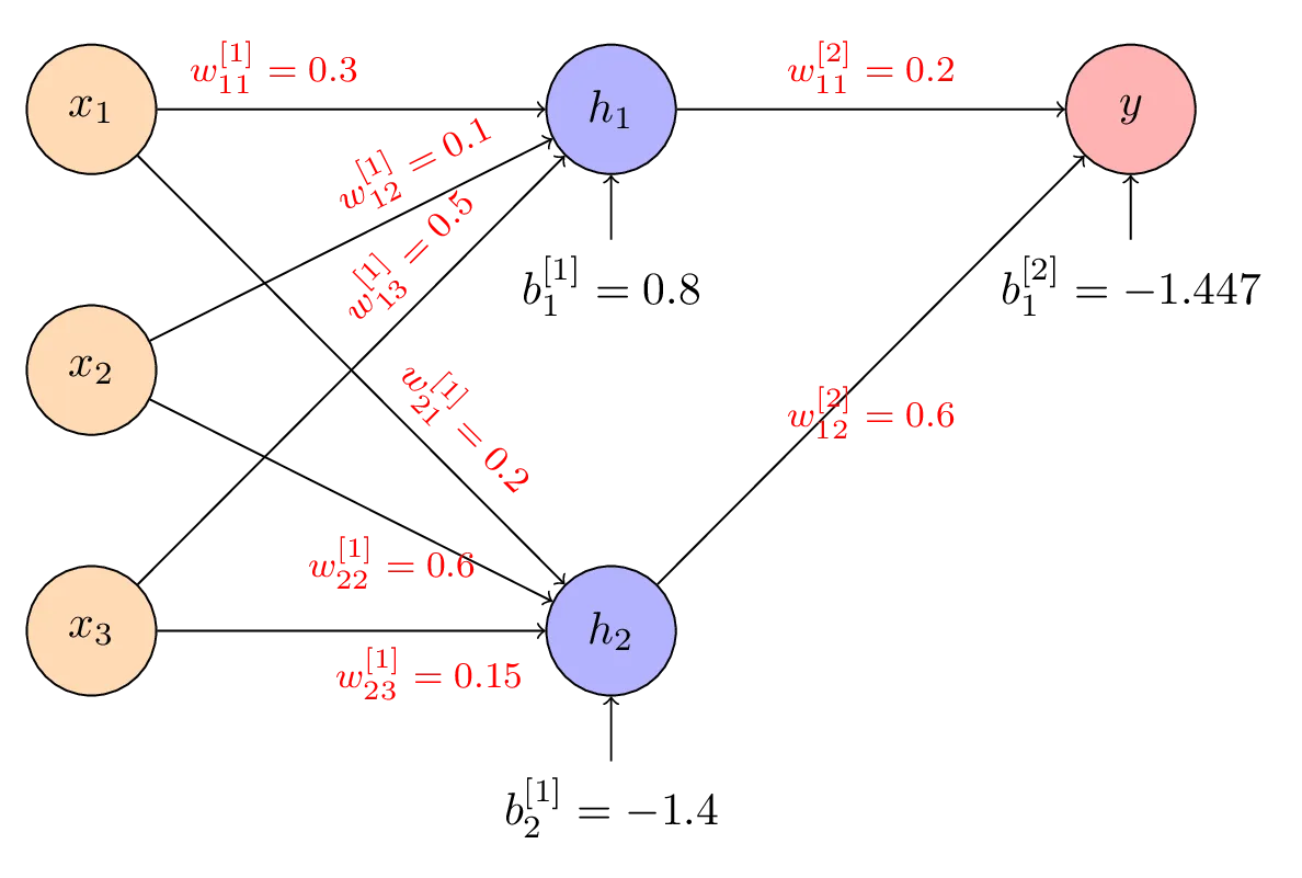
Solution

We calculate the weighted sum for the first hidden neuron:

$$z = w_{11}^{[1]} x_1 + w_{12}^{[1]} x_2 + w_{13}^{[1]} x_3 + b_1^{[1]} = (0.3)(1.2) + (0.1)(0.05) + (0.5)(0.6530) + 0.8 = 1.4915$$

Then we apply the sigmoid activation function:

$$a_1^{[1]} = \sigma(1.4915) = \frac{1}{1 + e^{-1.4915}} \approx 0.8163$$

(f) Compute $a_{2}^{[1]}$. Assume that $x_1 = 1.2, x_2 = 0.05$, $x_3 = 0.6530$ and use the sigmoid function for the activation function.

Solution

We calculate the weighted sum for the second hidden neuron:

$$z = w_{21}^{[1]} x_1 + w_{22}^{[1]} x_2 + w_{23}^{[1]} x_3 + b_2^{[1]} = (0.2)(1.2) + (0.6)(0.05) + (0.15)(0.6530) - 1.4 = -1.03205$$

Then we apply the sigmoid activation function:

$$a_2^{[1]} = \sigma(-1.03205) = \frac{1}{1 + e^{-(-1.03205)}} \approx 0.2627$$

(g) Compute the output of the above network, $y$. Assume that $x_1 = 1.2, x_2 = 0.05$, $x_3 = 0.6530$ and use the sigmoid function for the activation function.

Solution

We calculate the weighted sum for the output layer using the hidden layer activations:

$$z = w_{11}^{[2]} a_1^{[1]} + w_{12}^{[2]} a_2^{[1]} + b_1^{[2]} = (0.2)(0.8163) + (0.6)(0.2627) - 1.447 = -1.12612$$

Then we apply the sigmoid function to get the final output:

$$y = a_1^{[2]} = \sigma(-1.12612) = \frac{1}{1 + e^{-(-1.12612)}} \approx 0.2449$$

Problem 5: Grayscaling

In this question we will review grayscaling.

(a) What is a pixel?

Solution

A pixel is the smallest unit in a digital screen or display. Each pixel can only show one color at any given time.

(b) True or False? The RGB color model states that red, green and blue can be combined in different ways to produce a wide range of colors.

Solution

True. In the RGB model, any color can be represented as a linear combination of red, green, and blue.

(c) What is your favorite color?

Solution

My favorite color is turquoise.

(d) Using this site, http://www.cknuckles.com/rgbsliders.html, find out the RGB values for the color you picked above. Note: You’re welcome to use any other website that has a RGB slider such as this one: https://tuneform.com/tools/color/rgb-color-creator.

Solution

For turquoise, the RGB values are $(64, 224, 208)$.

(e) What formula did we use to convert a color to grayscale? Hint: https://en.wikipedia.org/wiki/Luma_(video)#Rec._601_luma_versus_Rec._709_luma_coefficients.

Solution

The Luminosity Method formula is used to convert a color to grayscale: $0.2989r + 0.5870g + 0.1140b$.

(f) Using the formula above, convert the RGB value of your favorite color in part (c) to grayscale. Write down what value of red, green and blue you get.

Solution

Applying the Luminosity Method:

$$0.2989(64) + 0.5870(224) + 0.1140(208) = 174.2496 \approx 174$$

So the grayscale RGB values are $(174, 174, 174)$.

(g) For the color you get above, what is the grayscale intensity? (Hint: just divide by 255).

Solution

The grayscale intensity is $\frac{174}{255} \approx 0.6824$.

Problem 6: Neural Network Overview

In this question we will review the final product — our neural network.

(a) Write down the four steps in creating a neural network.

Solution

The four steps are:

1. Define the input and output layers based on your problem
2. Choose the number of hidden layers and the number of neurons in each
3. Select cost and activation functions
4. Use training data with a training algorithm (such as mini-batch gradient descent) to determine the optimal weights and biases

(b) For the neural network example we considered in class, what was our task?

Solution

The task was to recognize and classify handwritten digits (0 through 9) from images.

(c) We stated that the inputs were pictures but to be more precise, we needed these inputs to be numerical. How did we get the images to be numerical?

Solution

We converted images to numerical form by assigning grayscale values to each of the $28 \times 28 = 784$ pixels in each image.

(d) How many layers did our neural network have?

Solution

Our neural network had 3 layers: the input layer, the hidden layer, and the output layer.

(e) Within each layer, how many neurons did we have?

Solution

The input layer had $28 \times 28 = 784$ neurons (one for each pixel). The hidden layer had 30 neurons, and the output layer had 10 neurons (one for each digit 0 through 9).

(f) What do we hope the hidden layer is doing?

Solution

We hope the hidden layer learns to function as a feature detector, enabling its neurons to recognize specific patterns in handwritten digits, such as horizontal strokes found in digits like 7.

(g) What activation function did we use?

Solution

We used the sigmoid function as the activation function.

(h) How did we find the weights and biases?

Solution

We determined the weights and biases using mini-batch gradient descent.

Problem 7: Running a Neural Network on MNIST

In this question we will run an image through the neural network we saw in class. Please note that you do not have to enter any code; instead, you’re just running code that I will provide.

(a) Download the image on Brightspace called “homework_image”.

Solution

(Solution involves downloading an image file.)

(b) Click this link: https://colab.research.google.com/drive/1s0SaR8cYUf52jumFDt26Xe0nj6ORVOUd?usp=sharing. You wouldn’t be able to edit this code since this is located in my Google Drive. You’ll need to save a copy of this in your own Drive. To do so, click “File” followed by “Save a Copy in Drive”.

Solution

(Solution involves accessing and copying a Google Colab notebook.)

(c) Execute the first three cells. It should take about 8 minutes. Upon executing the third cell, you will be prompted to upload an image. Upload the image you downloaded from Brightspace called “homework_image”.

Solution

(Solution involves executing code cells and uploading an image.)

(d) Execute the remaining cell blocks and make a note of the probabilities you obtain in the last code block. What does the neural network predict the digit is?

Solution

The neural network predicted the digit 3.

(e) Redo parts (c) and (d) again. Did you get a different result or different probabilities?

Solution

Upon redoing parts (c) and (d), the network still predicted digit 3, but the probabilities changed. In the second run, I got higher probabilities for digits 1 and 2 than originally, whereas in the first run the digit 5 had a nonzero probability. Digit 3 still maintained the highest probability across both runs, though its value was not constant.

(f) Above, you should get slightly different results each time. Can you perhaps explain why?

Solution

The variation in results is due to two reasons. First, when initializing the neural network, random weights and biases are generated each time. Second, the training process uses mini-batch gradient descent rather than batch gradient descent, which means the training data is randomly shuffled at the beginning of each epoch. Since the network trains on randomly selected mini-batches of images, the final weight values differ between runs. These differing weights lead to the slight variations in the output probabilities for different digits that we observe.

Problem 8: Deep Learning at Apple

For this question, please read the section called Introduction here: https://machinelearning.apple.com/research/face-detection.

(a) What kind of neural network does Apple use for features such as face recognition?

Solution

Apple uses Deep Neural Networks for features such as face recognition.

(b) What are the drawbacks of using models in deep learning? Hint: see the second paragraph under the section Introduction.

Solution

Deep learning models consume significant system resources compared to traditional computer vision. These models demand substantially more memory, disk storage, and computational power.

(c) How did Apple (and the rest of the industry) manage to overcome the drawbacks outlined above?

Solution

Apple and other companies addressed these limitations by using cloud-based services and APIs to execute their deep learning models. This approach enables them to send images to remote servers for analysis using deep learning inference. Since cloud services typically provide powerful GPUs with substantial memory capacity, they can run large deep learning models server-side rather than locally, making the technology accessible despite mobile devices being less powerful.