Math 245 Spring 2025 Exam 1

Formulas

1. Sigmoid Function:

   $$\sigma(z) = \frac{1}{1 + e^{-z}}$$

2. Mean Squared Error:

   $$\text{MSE} = \frac{1}{n}\sum_{i=1}^{n}(y_i - \hat{y}_i)^2$$

3. Luminosity Formula (grayscale conversion):

   $$0.2989r + 0.5870g + 0.1140b$$

4. (Half) Squared Euclidean Distance:

   $$C = \frac{1}{2}\sum_{i=1}^{n}(a_i - y_i)^2$$

5. Gradient Descent Algorithm (for two variables):

   (a) Initialize $x_{\text{old}}$ and $y_{\text{old}}$

   (b) Calculate $f(x_{\text{old}}, y_{\text{old}})$

   (c) Compute $\frac{\partial f}{\partial x}$ and $\frac{\partial f}{\partial y}$ at $(x_{\text{old}}, y_{\text{old}})$

   (d) Define $\alpha$ (learning rate)

   (e) Update the parameters:

   $$x_{\text{new}} = x_{\text{old}} - \alpha\frac{\partial f}{\partial x}(x_{\text{old}}, y_{\text{old}})$$ $$y_{\text{new}} = y_{\text{old}} - \alpha\frac{\partial f}{\partial y}(x_{\text{old}}, y_{\text{old}})$$

   (f) Repeat until convergence

Problem 1

These questions are conceptual (short answer) questions.

(a) [5 pt / 5 pts] Explain what is meant by a mathematical model.

Solution

A model that has numerical inputs and outputs.

(b) [5 pt / 10 pts] Consider Tom Mitchell’s definition of machine learning. If the task is to create a recommendation system for YouTube videos, then what can the training data be?

Solution

$$\mathbb{D} = \{(x_i, y_i)\}$$

where

$$x_i = \begin{bmatrix} \text{hours spent on YouTube} \\ \text{probability of liking sports} \\ \text{avg length of videos watched} \end{bmatrix}$$

and $y_i \in \{0, 1\}$ where 0 indicates the user did not click a recommended video and 1 indicates the user clicked a recommended video.

(c) [10 pt / 20 pts] Explain why the cost function can be considered a measure of error.

Solution

For us, the cost function usually has a $y_i - \hat{y}_i$ term, and this is exactly the error. We square the error and take the mean, so every cost function measures error because it has this error term.

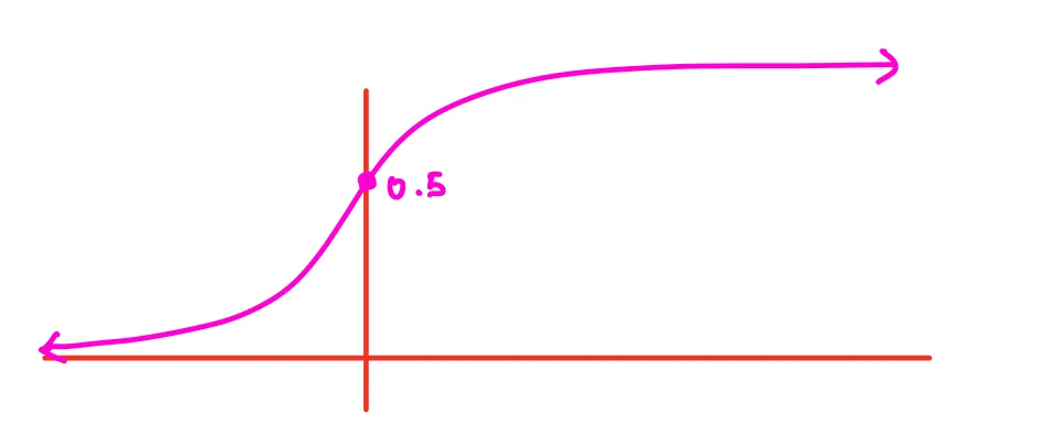
(d) [10 pt / 30 pts] Explain why continuous activation functions (such as the sigmoid function) are preferred over discrete activation functions (such as the perceptron activation function).

Solution

Continuous activations are preferred over discrete because the main problem with the perceptron is that small changes in the weights or biases produce large changes in the output. Continuous activation functions allow small changes in the weights and biases to produce small changes in the output. Additionally, continuous functions like the sigmoid are differentiable everywhere, which allows for gradient-based learning. In order to optimize, we have to take derivatives, and we get that with continuous activation functions but not with the perceptron.

Problem 2

Suppose we are given the following data: $(1, 5.15)$, $(5, 16.54)$, $(6, 20.04)$, $(7, 22.86)$.

(a) [5 pt / 35 pts] Further suppose we wish to model the above data via a linear function of the form $\hat{y}_i = 2x_i + 1$. Find $\hat{y}_i$ for $i = 1, 2, 3, 4$.

Solution

$$\begin{align*} \hat{y}_1 &= 2(1) + 1 = 3 \\ \hat{y}_2 &= 2(5) + 1 = 11 \\ \hat{y}_3 &= 2(6) + 1 = 13 \\ \hat{y}_4 &= 2(7) + 1 = 15 \end{align*}$$

(b) [5 pt / 40 pts] In class, our cost function was typically the mean squared error. Instead, let’s use a new cost function called the Mean Absolute Error or MAE. By definition,

$$\text{MAE} = \frac{1}{n} \sum_{i=1}^{n} |y_i - \hat{y}_i|$$

For the data in Problem 2(a) above, compute the Mean Absolute Error.

Solution

$x_i$	$y_i$	$\hat{y}_i$	$\vert y*i - \hat{y}*{i} \vert$
1	5.15	3	2.15
5	16.54	11	5.54
6	20.04	13	7.04
7	22.86	15	7.86

$$\text{MAE} = \frac{1}{4}(2.15 + 5.54 + 7.04 + 7.86) = 5.6475$$

Note: Both MSE and MAE have the $y_i - \hat{y}_i$ term. The difference is that MSE uses the square while MAE uses absolute value. MSE is easier to work with in practice because the squared term is always differentiable everywhere, whereas the absolute value function is not differentiable at certain points. Therefore, in practice you typically use MSE over MAE.

Problem 3

Consider the two-dimensional cost function below:

$$f(x, y) = (x - 4)^2 + (y + 3)^2$$

Note that the partial derivatives are:

$$\frac{\partial f}{\partial x} = 2(x - 4), \quad \frac{\partial f}{\partial y} = 2(y + 3)$$

(a) [15 pt / 55 pts] Perform the next two iterations of gradient descent starting at $(x_0, y_0) = (1, -1)$ with a learning rate of $\alpha = 0.5$.

Solution

Iteration 1

Starting with $x_0 = 1$, $y_0 = -1$:

$$f(1, -1) = (1 - 4)^2 + (-1 + 3)^2 = 9 + 4 = 13$$

Compute the partial derivatives:

$$f_x(1, -1) = 2(1 - 4) = -6$$ $$f_y(1, -1) = 2(-1 + 3) = 4$$

Update with $\alpha = 0.5$:

$$x_1 = 1 - 0.5(-6) = 4$$ $$y_1 = -1 - 0.5(4) = -3$$

Thus $(x_1, y_1) = (4, -3)$

Iteration 2

Starting with $x_1 = 4$, $y_1 = -3$:

$$f(4, -3) = 0$$

Compute the partial derivatives:

$$f_x(4, -3) = 0$$ $$f_y(4, -3) = 0$$

Update with $\alpha = 0.5$:

$$x_2 = 4 - 0.5(0) = 4$$ $$y_2 = -3 - 0.5(0) = -3$$

Thus $(x_2, y_2) = (4, -3)$

(b) [5 pt / 60 pts] Do you think this setup (meaning the initialization and learning rate specified above) will converge to a local minimum or global minimum?

Solution

This setup seems to have converged to a global minimum. Since $(x-4)^2$ is globally minimized when $x=4$ and $(y+3)^2$ is globally minimized when $y=-3$, the function converges to the global minimum.

Problem 4

Consider the following neural network.

(a) [10 pt / 70 pts] Assuming that $x_1 = 1$, $x_2 = 1$, and that the activation function is the sigmoid function, find $a^{[1]}_2$. You may round to two decimal places.

Solution

$$\sigma(0.2(1) + 0.5(1) + 0.2) = \sigma(0.9) = \frac{1}{1 + e^{-0.9}} \approx 0.71$$

Problem 5

In class, we discussed (regular) gradient descent versus mini-batch gradient descent.

(a) [5 pt / 75 pts] When is it suitable to use mini-batch gradient descent instead of (regular) gradient descent?

Solution

When our dataset is extremely large.

(b) [5 pt / 80 pts] Which method is inherently more random? Explain why.

Solution

Mini-batch GD is more random because there is variability in how the data is being shuffled in. This doesn’t happen in (batch) GD since in (batch) GD, we update over the ENTIRE dataset.

Problem 6

In class, we discussed how convergence in gradient descent depends on initialization and the learning rate. Depending on these factors, gradient descent can converge to different points. Assume that the cost function, $C(m, b)$, is known and consider the following situation:

(a) [10 pt / 90 pts] Both Alice and Bob see the same data set and use the same cost function. Alice implements the gradient descent algorithm with an initialization at $(0, 0)$ and a learning rate of $1$. By the end of the gradient descent process, she converges to $m = 2$ and $b = 4$. Meanwhile, Bob initializes at $(245, 245)$ with a learning rate of $3$ and converges to $m = 1$ and $b = -1$. How can we determine which point is more likely to yield the global minimum?

Solution

Compute $C(2, 4)$ vs. $C(1, -1)$. Whichever has the lower cost is more likely to be the global minimum.

Problem 7

This question will ask you to summarize our discussion from class.

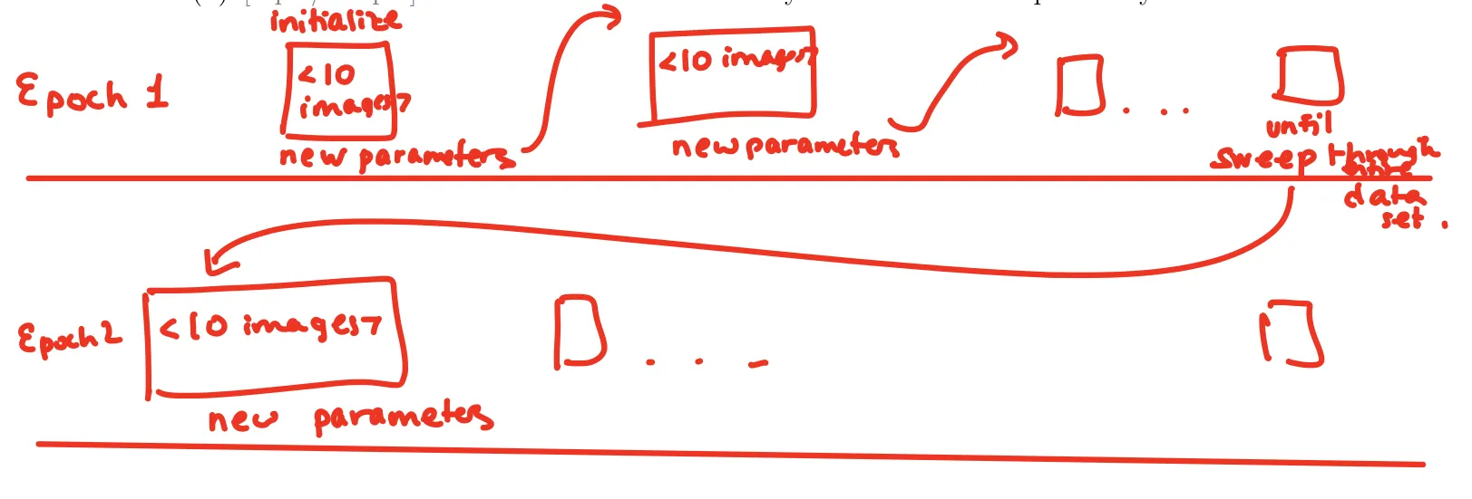
(a) [10 pt / 100 pts] Explain how a feedforward neural network can classify MNIST digits. Points will be awarded based on the clarity and completeness of your answer. Your answer should include the terms: task, training data, grayscale, input layer, output layer, hidden layer, mini-batch gradient descent, epoch, cost function, feature detection, and neural network.

Solution

Our task is to classify a handwritten digit. Our model is a neural network. Our neural network consists of an input layer, output layer, and hidden layer. The input layer takes the grayscale intensity of each pixel, the hidden layer detects features, and the output layer represents the activations for every digit.

Our training data consists of 50,000 images from the MNIST dataset where each picture is a 28×28 grayscaled photo of a digit. Since there is a large amount of data, we’ll aim to use mini-batch gradient descent, where we feed in (let’s say) 10 images at a time and run gradient descent with our cost function on just these 10 images. Doing this 5,000 times sweeps through the entire dataset, which is a single epoch. We’ll then repeat this over multiple epochs until the cost function converges.