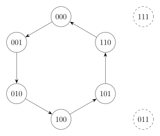
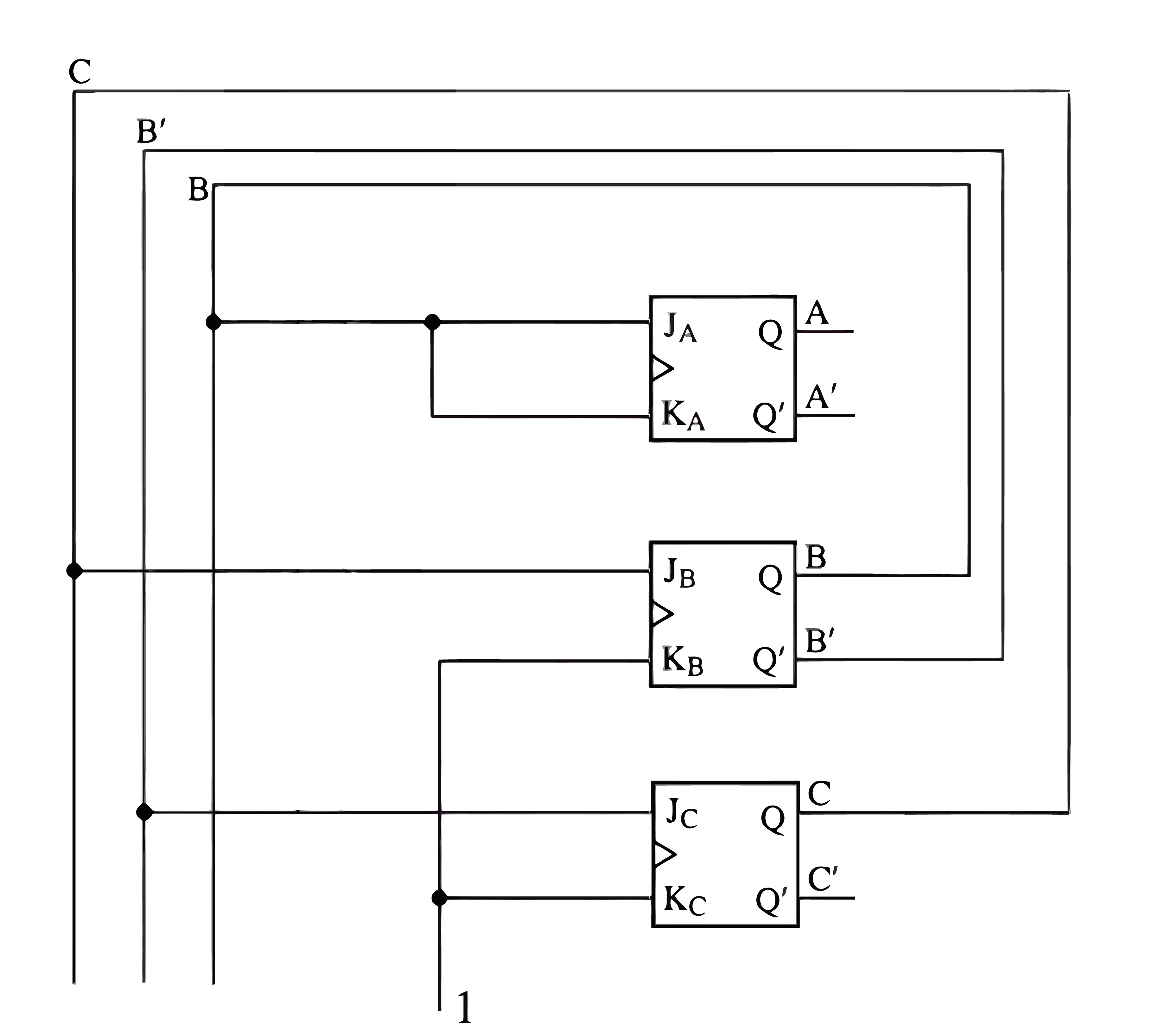
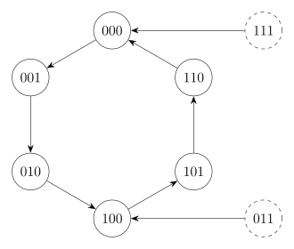
A non-binary counter is a synchronous counter that cycles through a subset of states, skipping others. In this example, we design a counter for the following sequence using JK flip-flops:
0 → 1 → 2 → 4 → 5 → 6 → 0 → ⋯ 0 \to 1 \to 2 \to 4 \to 5 \to 6 \to 0 \to \cdots 0 → 1 → 2 → 4 → 5 → 6 → 0 → ⋯ States 3 (011) and 7 (111) are missing from the sequence, so they are the unused states for this counter. When drawing the state diagram, we have the option to include them as nodes but with no transitions leading into them, since they’re unused — we treat them as don’t-care conditions in the K-maps.
We first lay out the state table for the desired transitions:
Q ( t ) Q ( t + 1 ) f/f Inputs A B C A B C J A K A J B K B J C K C 0 0 0 0 0 1 0 0 1 0 1 0 0 1 0 1 0 0 1 0 0 1 0 1 1 0 1 1 1 0 1 1 0 0 0 0 \begin{array}{ccc|ccc|cccccc}
& Q(t) & & & Q(t{+}1) & & & & \text{f/f} & \text{Inputs} & & \\
\hline
A & B & C & A & B & C & J_A & K_A & J_B & K_B & J_C & K_C \\
\hline
0 & 0 & 0 & 0 & 0 & 1 & & & & & & \\
0 & 0 & 1 & 0 & 1 & 0 & & & & & & \\
0 & 1 & 0 & 1 & 0 & 0 & & & & & & \\
1 & 0 & 0 & 1 & 0 & 1 & & & & & & \\
1 & 0 & 1 & 1 & 1 & 0 & & & & & & \\
1 & 1 & 0 & 0 & 0 & 0 & & & & & & \\
\end{array} A 0 0 0 1 1 1 Q ( t ) B 0 0 1 0 0 1 C 0 1 0 0 1 0 A 0 0 1 1 1 0 Q ( t + 1 ) B 0 1 0 0 1 0 C 1 0 0 1 0 0 J A K A f/f J B Inputs K B J C K C The JK flip-flop’s excitation table tells us the required J and K inputs for any given Q ( t ) → Q ( t + 1 ) Q(t) \to Q(t{+}1) Q ( t ) → Q ( t + 1 )
Q ( t ) Q ( t + 1 ) J K 0 0 0 X 0 1 1 X 1 0 X 1 1 1 X 0 \begin{array}{cc|cc}
Q(t) & Q(t+1) & J & K \\
\hline
0 & 0 & 0 & X \\
0 & 1 & 1 & X \\
1 & 0 & X & 1 \\
1 & 1 & X & 0 \\
\end{array} Q ( t ) 0 0 1 1 Q ( t + 1 ) 0 1 0 1 J 0 1 X X K X X 1 0 We apply the JK excitation table to determine the required J and K inputs for each flip-flop in each state transition:
Q ( t ) Q ( t + 1 ) f/f Inputs A B C A B C J A K A J B K B J C K C 0 0 0 0 0 1 0 X 0 X 1 X 0 0 1 0 1 0 0 X 1 X X 1 0 1 0 1 0 0 1 X X 1 0 X 1 0 0 1 0 1 X 0 0 X 1 X 1 0 1 1 1 0 X 0 1 X X 1 1 1 0 0 0 0 X 1 X 1 0 X \begin{array}{ccc|ccc|cccccc}
& Q(t) & & & Q(t{+}1) & & & & \text{f/f} & \text{Inputs} & & \\
\hline
A & B & C & A & B & C & J_A & K_A & J_B & K_B & J_C & K_C \\
\hline
0 & 0 & 0 & 0 & 0 & 1 & 0 & X & 0 & X & 1 & X \\
0 & 0 & 1 & 0 & 1 & 0 & 0 & X & 1 & X & X & 1 \\
0 & 1 & 0 & 1 & 0 & 0 & 1 & X & X & 1 & 0 & X \\
1 & 0 & 0 & 1 & 0 & 1 & X & 0 & 0 & X & 1 & X \\
1 & 0 & 1 & 1 & 1 & 0 & X & 0 & 1 & X & X & 1 \\
1 & 1 & 0 & 0 & 0 & 0 & X & 1 & X & 1 & 0 & X \\
\end{array} A 0 0 0 1 1 1 Q ( t ) B 0 0 1 0 0 1 C 0 1 0 0 1 0 A 0 0 1 1 1 0 Q ( t + 1 ) B 0 1 0 0 1 0 C 1 0 0 1 0 0 J A 0 0 1 X X X K A X X X 0 0 1 f/f J B 0 1 X 0 1 X Inputs K B X X 1 X X 1 J C 1 X 0 1 X 0 K C X 1 X X 1 X States 3 (011) and 7 (111) are unused — they are treated as don’t-care conditions (X X X
If we wanted, we could include them in the table — their flip-flop input entries would just be all don’t-cares:
Q ( t ) Q ( t + 1 ) f/f Inputs A B C A B C J A K A J B K B J C K C 0 0 0 0 0 1 0 X 0 X 1 X 0 0 1 0 1 0 0 X 1 X X 1 0 1 0 1 0 0 1 X X 1 0 X 0 1 1 X X X X X X X X X 1 0 0 1 0 1 X 0 0 X 1 X 1 0 1 1 1 0 X 0 1 X X 1 1 1 0 0 0 0 X 1 X 1 0 X 1 1 1 X X X X X X X X X \begin{array}{ccc|ccc|cccccc}
& Q(t) & & & Q(t{+}1) & & & & \text{f/f} & \text{Inputs} & & \\
\hline
A & B & C & A & B & C & J_A & K_A & J_B & K_B & J_C & K_C \\
\hline
0 & 0 & 0 & 0 & 0 & 1 & 0 & X & 0 & X & 1 & X \\
0 & 0 & 1 & 0 & 1 & 0 & 0 & X & 1 & X & X & 1 \\
0 & 1 & 0 & 1 & 0 & 0 & 1 & X & X & 1 & 0 & X \\
{\color{red}0} & {\color{red}1} & {\color{red}1} & X & X & X & X & X & X & X & X & X \\
1 & 0 & 0 & 1 & 0 & 1 & X & 0 & 0 & X & 1 & X \\
1 & 0 & 1 & 1 & 1 & 0 & X & 0 & 1 & X & X & 1 \\
1 & 1 & 0 & 0 & 0 & 0 & X & 1 & X & 1 & 0 & X \\
{\color{red}1} & {\color{red}1} & {\color{red}1} & X & X & X & X & X & X & X & X & X \\
\end{array} A 0 0 0 0 1 1 1 1 Q ( t ) B 0 0 1 1 0 0 1 1 C 0 1 0 1 0 1 0 1 A 0 0 1 X 1 1 0 X Q ( t + 1 ) B 0 1 0 X 0 1 0 X C 1 0 0 X 1 0 0 X J A 0 0 1 X X X X X K A X X X X 0 0 1 X f/f J B 0 1 X X 0 1 X X Inputs K B X X 1 X X X 1 X J C 1 X 0 X 1 X 0 X K C X 1 X X X 1 X X
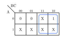
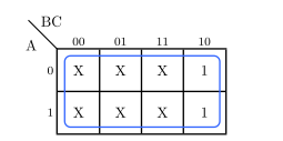
J A : J_A: J A :
J A = B J_A = B J A = B
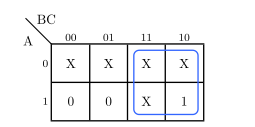
K A : K_A: K A :
K A = B K_A = B K A = B
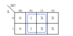
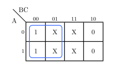
J B : J_B: J B :
J B = C J_B = C J B = C
K B : K_B: K B :
K B = 1 K_B = 1 K B = 1
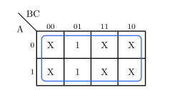
J C : J_C: J C :
J C = B ′ J_C = B' J C = B ′
K C : K_C: K C :
K C = 1 K_C = 1 K C = 1
To check whether the circuit is self-correcting, we plug each unused state into the derived flip-flop expressions and trace where the circuit goes next. As with the S/R case covered previously, we interpret the resulting J/K values according to the flip-flop’s characteristic behavior: J = 0 , K = 0 J=0, K=0 J = 0 , K = 0 J = 1 , K = 0 J=1, K=0 J = 1 , K = 0 J = 0 , K = 1 J=0, K=1 J = 0 , K = 1 J = 1 , K = 1 J=1, K=1 J = 1 , K = 1
J A = B J B = C J C = B ′ K A = B K B = 1 K C = 1 \begin{aligned}
J_A &= B \quad & J_B &= C \quad & J_C &= B' \\
K_A &= B \quad & K_B &= 1 \quad & K_C &= 1
\end{aligned} J A K A = B = B J B K B = C = 1 J C K C = B ′ = 1 Unused state ABC = 011:
J A = B = 1 K A = B = 1 ⇒ complement A ( 0 → 1 ) J B = C = 1 K B = 1 ⇒ complement B ( 1 → 0 ) J C = B ′ = 0 K C = 1 ⇒ reset C to 0 \begin{aligned}
J_A &= B = 1 \quad & K_A &= B = 1 & &\Rightarrow \text{complement } A \text{ (}0 \to 1\text{)} \\
J_B &= C = 1 & K_B &= 1 & &\Rightarrow \text{complement } B \text{ (}1 \to 0\text{)} \\
J_C &= B' = 0 & K_C &= 1 & &\Rightarrow \text{reset } C \text{ to } 0
\end{aligned} J A J B J C = B = 1 = C = 1 = B ′ = 0 K A K B K C = B = 1 = 1 = 1 ⇒ complement A ( 0 → 1 ) ⇒ complement B ( 1 → 0 ) ⇒ reset C to 0 011 → 100 011 \to 100 011 → 100 State 100 is valid, so the circuit self-corrects out of state 011.
Unused state ABC = 111:
J A = B = 1 K A = B = 1 ⇒ complement A ( 1 → 0 ) J B = C = 1 K B = 1 ⇒ complement B ( 1 → 0 ) J C = B ′ = 0 K C = 1 ⇒ reset C to 0 \begin{aligned}
J_A &= B = 1 \quad & K_A &= B = 1 & &\Rightarrow \text{complement } A \text{ (}1 \to 0\text{)} \\
J_B &= C = 1 & K_B &= 1 & &\Rightarrow \text{complement } B \text{ (}1 \to 0\text{)} \\
J_C &= B' = 0 & K_C &= 1 & &\Rightarrow \text{reset } C \text{ to } 0
\end{aligned} J A J B J C = B = 1 = C = 1 = B ′ = 0 K A K B K C = B = 1 = 1 = 1 ⇒ complement A ( 1 → 0 ) ⇒ complement B ( 1 → 0 ) ⇒ reset C to 0 111 → 000 111 \to 000 111 → 000 State 000 is valid, so the circuit also self-corrects out of state 111.
With the self-correction transitions now known, we can complete the state diagram by adding the transitions out of the unused states: