Lec 04-30-2026: Lines & Planes (cont.) & Support Vector Machines

Lines & Planes (cont)

(Ending of our Linear Algebra recap)

In our last lecture, we introduced the notion of a hyperplane. Recall that a hyperplane is a flat $(n-1)$-dimensional surface in $\mathbb{R}^n$ - a line in $\mathbb{R}^2$, a flat plane in $\mathbb{R}^3$, and so on. Algebraically, a hyperplane is given by $\vec{w}^T\vec{x} + b = 0$:

$$\begin{bmatrix} w_1 & w_2 & \cdots & w_n \end{bmatrix} \begin{bmatrix} x_1 \\ x_2 \\ \vdots \\ x_n \end{bmatrix} + b = 0$$ $$w_1x_1 + w_2x_2 + \cdots + w_nx_n + b = 0$$

Intuition

A hyperplane is just a generalization of a 2D line to higher dimensions!

In 2D, this becomes $w_1x_1 + w_2x_2 + b = 0$. Rearranging to isolate $x_2$ (which plays the role of $y$):

$$w_2x_2 = -w_1x_1 - b \implies x_2 = \frac{-w_1}{w_2}x_1 - \frac{b}{w_2} \implies y = mx + b$$

Note: the "$b$" in slope-intercept form here is $-b/w_2$, which is a different value from the $b$ in the original hyperplane equation - they just happen to share the same letter.

Theorem: $\vec{w}$ is Orthogonal to the Hyperplane

Theorem

For every hyperplane $\vec{w}^T\vec{x} + b = 0$, the vector $\vec{w}$ is always orthogonal to our hyperplane.

Proof

To show $\vec{w}$ is orthogonal to the entire hyperplane, it suffices to show it is orthogonal to any vector lying parallel to the hyperplane (since such vectors span all directions within the hyperplane). Let $\vec{v}$ be an arbitrary vector parallel to the hyperplane, with $\vec{v}_1$ & $\vec{v}_2$ pointing from the origin to the base & tip of $\vec{v}$ respectively.

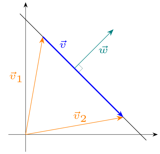
Since $\vec{v}_1$ & $\vec{v}_2$ begin from the origin, we have:

$$\vec{v} = \vec{v}_2 - \vec{v}_1 \quad \text{(parallel to hyperplane)}$$

Since the tips of $\vec{v}_1$ & $\vec{v}_2$ lie on the hyperplane $\vec{w}^T\vec{x} + b = 0$, they each satisfy the hyperplane equation:

$$\vec{w}^T\vec{v}_2 + b = 0 \qquad \text{and} \qquad \vec{w}^T\vec{v}_1 + b = 0$$

Subtracting the second equation from the first eliminates $b$, leaving:

$$\vec{w}^T\vec{v}_2 - \vec{w}^T\vec{v}_1 = 0 \implies \vec{w}^T(\vec{v}_2 - \vec{v}_1) = 0 \implies \vec{w}^T\vec{v} = 0$$

Recall

If the dot product is 0, then this means the vectors are orthogonal to each other.

Hence $\vec{w}$ is orthogonal to $\vec{v}$. Since $\vec{v}$ is parallel to the hyperplane, then $\vec{w}$ is also orthogonal to the hyperplane. $\square$

Corollary

(Another structure of math)

Corollary

$\dfrac{1}{\|\vec{w}\|}\vec{w} = \hat{w}$ is also orthogonal to the hyperplane $\vec{w}^T\vec{x} + b = 0$.

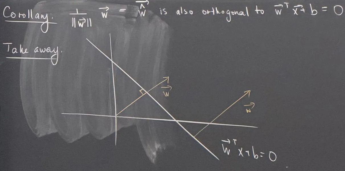
This follows immediately from the theorem: $\hat{w}$ is just $\vec{w}$ scaled by the positive scalar $\frac{1}{\|\vec{w}\|}$, so it points in the exact same direction as $\vec{w}$. Since orthogonality depends only on direction, $\hat{w}$ is orthogonal to the hyperplane too.

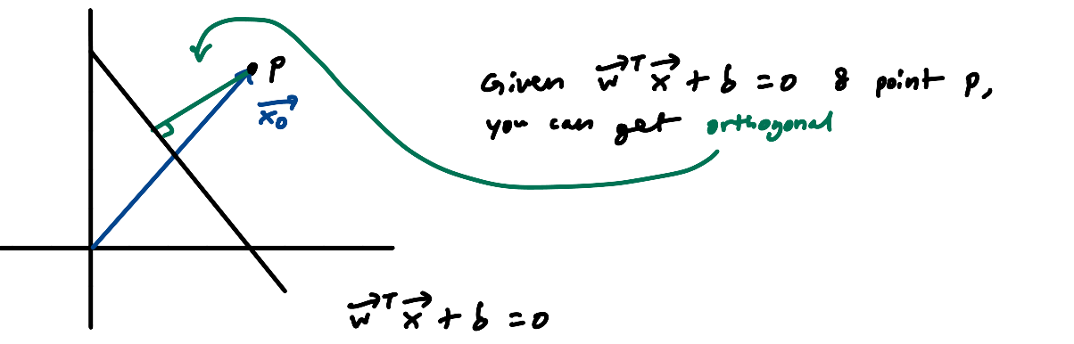
Take Away

By default, we draw $\vec{w}$ with its tail at the origin. However, since $\vec{w}$ represents a direction (perpendicular to the hyperplane), we can translate it to start from any point and it still correctly describes the orientation of the hyperplane - as the diagram below illustrates.

Distance from a Point to a Hyperplane

Given a point $P$ not on the hyperplane, we want the shortest distance from $P$ to the hyperplane. As before, the hyperplane is defined by $\vec{w}^T\vec{x} + b = 0$.

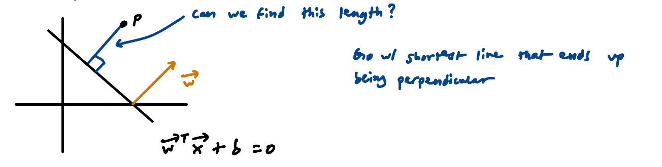
There are infinitely many line segments connecting $P$ to some point on the hyperplane, but the shortest one is always the perpendicular one. (Any non-perpendicular segment forms the hypotenuse of a right triangle whose leg includes the perpendicular segment, making it strictly longer.) So we go with the perpendicular segment.

Setting Up Variables

Step 1: Project P onto the hyperplane:

• Call the vector from the origin to the projection of $P$: $\vec{x}_p$
• Call the vector between $\vec{x}_p$ & $P$: $\vec{d}$
• Call the vector between the origin & $P$: $\vec{x}_0$

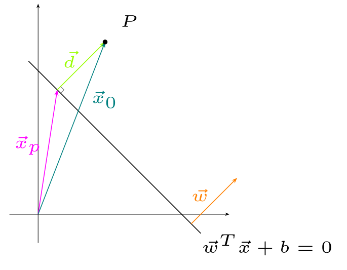
From the diagram:

$$\vec{x}_p + \vec{d} = \vec{x}_0 \implies \vec{x}_p = \vec{x}_0 - \vec{d} \tag{Eq 1}$$

Deriving the Distance

Since the tip of $\vec{x}_p$ lies on the hyperplane, then $\vec{w}^T\vec{x}_p + b = 0$.

Since $\vec{d}$ is the perpendicular segment from $P$ to the hyperplane, it is orthogonal to the hyperplane. But $\vec{w}$ is also orthogonal to the hyperplane. Two vectors that are both perpendicular to the same surface must be parallel to each other, so $\vec{d}$ is a scalar multiple of $\vec{w}$:

$$\vec{d} = s\vec{w} \tag{Eq 2}$$

Again our goal is to use this to find the length between P & the hyperplane, aka $\|\vec{d}\|$.

Substituting Eq 1 into $\vec{w}^T\vec{x}_p + b = 0$:

$$\begin{aligned} \vec{w}^T(\vec{x}_0 - \vec{d}) + b &= 0 \\ \vec{w}^T(\vec{x}_0 - s\vec{w}) + b &= 0 && \text{(Eq 2)} \\ \vec{w}^T\vec{x}_0 - s\vec{w}^T\vec{w} + b &= 0 \\ \vec{w}^T\vec{x}_0 + b &= s\vec{w}^T\vec{w} \\ s &= \frac{\vec{w}^T\vec{x}_0 + b}{\vec{w}^T\vec{w}} \tag{Eq 3} \end{aligned}$$

Since $\vec{d} = s\vec{w}$, by Eq 3:

$$\vec{d} = \left(\frac{\vec{w}^T\vec{x}_0 + b}{\vec{w}^T\vec{w}}\right)\vec{w}$$

Computing $\|\vec{d}\|$

Simplification to keep in mind

$\dfrac{\sqrt{c}}{c} = \dfrac{\sqrt{c}}{\sqrt{c}\,\sqrt{c}} = \dfrac{1}{\sqrt{c}}$

$$\begin{aligned} \|\vec{d}\| &= \sqrt{\vec{d}^T\vec{d}} \\ &= \sqrt{(s\vec{w})^T(s\vec{w})} \\ &= \sqrt{s\vec{w}^T \cdot s\vec{w}} \\ &= \sqrt{s^2\,\vec{w}^T\vec{w}} \\ &= \sqrt{s^2}\,\sqrt{\vec{w}^T\vec{w}} \\ &= |s|\sqrt{\vec{w}^T\vec{w}} \\ &= \left|\frac{\vec{w}^T\vec{x}_0 + b}{\vec{w}^T\vec{w}}\right|\sqrt{\vec{w}^T\vec{w}} \\ &= \frac{|\vec{w}^T\vec{x}_0 + b|}{\vec{w}^T\vec{w}}\,\sqrt{\vec{w}^T\vec{w}} && (\vec{w}^T\vec{w} \geq 0) \\ &= \frac{|\vec{w}^T\vec{x}_0 + b|}{\sqrt{\vec{w}^T\vec{w}}} = \frac{|\vec{w}^T\vec{x}_0 + b|}{\sqrt{\|\vec{w}\|^2}} = \frac{|\vec{w}^T\vec{x}_0 + b|}{\|\vec{w}\|} \end{aligned}$$

Distance Formula: Point to Hyperplane

Given $\vec{w}^T\vec{x} + b = 0$ & point $p$, the orthogonal distance from $p$ to the hyperplane is:

$$\|\vec{d}\| = \frac{|\vec{w}^T\vec{x}_0 + b|}{\|\vec{w}\|}$$

Support Vector Machines (SVM)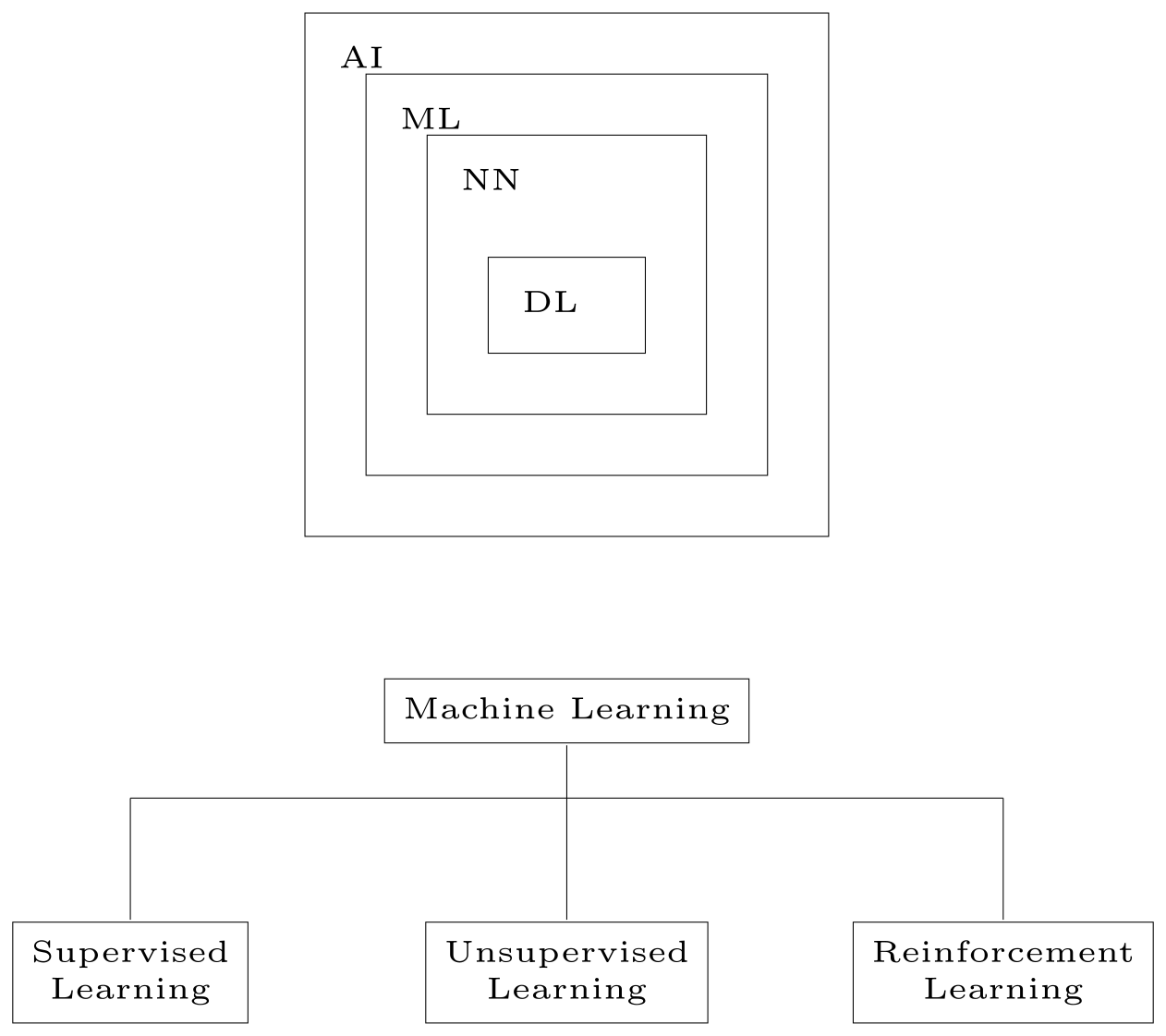

SVMs are a type of supervised learning.

Idea: Given a bunch of data points which belong to 1 of 2 classes, the goal is to decide which class a new datapoint will belong to.

Example: In medicine, a tumor is an abnormal growth of cells which may or may not be cancerous.

Wisconsin Breast Cancer Dataset (1995)

Let’s develop a model which can attempt to differentiate if a tumor is/isn’t cancerous based on the following training data.

Each patient’s data contains 13 features (size of tumor, cell density, length of tumor, …) and 1 label (C = cancerous, N = non-cancerous), giving 14 dimensions total. The data for patient $i$ is represented as $(\vec{x}_i, y_i)$ where $y_i \in \{C, N\}$ is encoded as $1$ or $-1$.

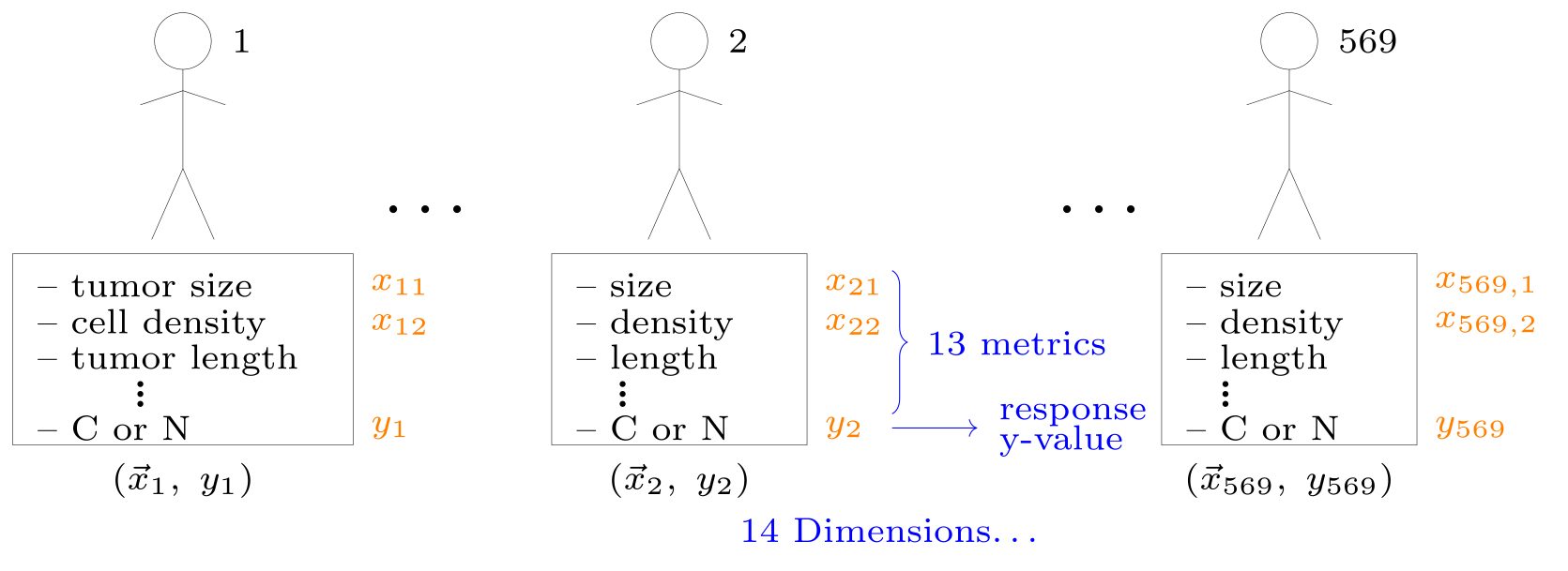
Each data point is a pair $(\vec{x}_i, y_i)$: a feature vector and a label. Since the output is categorical, we encode the label numerically:

$$\left(\underbrace{\begin{bmatrix}\text{tumor size}\\\text{cell density}\\\text{tumor length}\\\vdots\end{bmatrix}}_{\vec{x}_i},\; \underbrace{C \text{ or } N}_{1 \text{ or } -1}\right)$$

Let $X_{ij}$ denote the $j^{\text{th}}$ feature of patient $i$.

• $X_{11}$ is the first feature of patient (pt) 1.
• $X_{12}$ is the second feature of patient (pt) 1.
• $Y_1$ is either C or N.

Since cancerous tumors rapidly divide & grow uncontrollably, they tend to have measurable differences in properties like tumor size and cell density. The hypothesis is that a few of the 13 features can reliably discriminate between the two classes.

We’ll start with just 2 of the 13 features to visualize the idea, then generalize to all dimensions. The output we predict is the label $y_i \in \{+1, -1\}$ for a new patient.

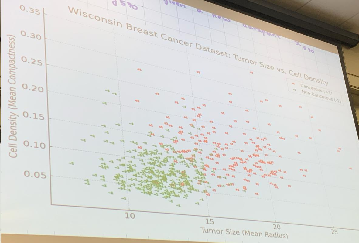
With 569 training patients plotted, now imagine a $570^{\text{th}}$ patient walks in. Their features give a new point on this scatter plot - the question is: which class does it belong to, and how do we draw the boundary that separates them?