Lecture 23: Space Complexity and Binary Tree Array Mapping - CSCI 381 Goldberg

Administrative Updates

Mostly same as TC20, but with some clarifications:

• Quiz – Wednesday, April 29: Covers only material from after spring break. The recursion lecture posted on March 25th is not included on any quiz (but may appear on the final).

• Review Day – Sunday, May 4: Open Q&A session focused on quiz questions. Students should come prepared with specific questions they want reviewed. The session is student-driven. Questions emailed to the class-designated email before Monday will be prioritized (first-come, first-served with round-robin fairness). Questions must be typed — no photo snapshots — so they can be incorporated into Excel.

Last Day of New Material

This is the last day of new material, and the last day covered by MCQ and lecture keywords — except for the research paper.

Introduction

Savitch’s Theorem

The following relationships hold in complexity theory:

• $\text{NSPACE}(f(n)) \subseteq \text{DSPACE}(f(n)^2)$ — Last class we applied this to $f(n) = \text{poly}(n)$. The intuition: a non-deterministic TM using $f(n)$ space produces a tableau with $f(n)$ rows (one per time step) and $f(n)$ columns (one per tape cell), for $f(n)^2$ total cells. A deterministic machine can simulate the non-deterministic computation by exhaustively trying every possible string of characters that fits in that tableau — one of those configurations will be the correct accepting path.

• $\text{DTIME}(f(n)) \subseteq \text{DSPACE}(f(n))$ — A Turing machine can only advance one cell (space) in a given clock step

• $\text{DSPACE}(f(n)) \subseteq \text{DTIME}(2^{f(n)})$ — Exhaustive search (brute-force) of a fixed size memory could generate an exponential amount of different values, one (or more) of which is the solution to your problem

“Put a monkey in a room with a typewriter and eventually it will type out Shakespeare.” — Émile Borel (1913)

Relating Turing Machines to RAM

In the tableau we used for Savitch’s theorem, we superimposed an index to the cells of the tape. This was enabled by the fact that we were considering a variant of the Turing machine where the tape is infinite in only one direction. As such, the first cell (on left) has index 0 and we can sequentially (uniquely) assign an index to all subsequent cells of the tape.

This is very similar to what we call RAM (Random Access Memory). Random access memory allows the operating system to go directly in $O(1)$ time to a given position in the memory based on a single address. If the above “index” was truly like how we consider an index to an array, then our simulation for Savitch’s theorem was like using RAM. The fact is that our proof didn’t actually require this because Turing machine tapes can be addressed and accessed as in RAM, but just not in constant time. One could specify an address and then advance the tape that many cells.

However, the efficiency gained by having addressing achieved in constant time gave some in the literature cause to consider a true RAM variant of a Turing machine: A Turing machine where the “tape advances” in constant time to a given address. (If need be, then this variant would replace the tape concept with linear memory chips as we have now.)

Now that everything is stored in this linear array of memory (whether hardware or tape), this brings up the issue of how multi-dimensional data structures can be stored in such a Turing machine:

• 2D Array / Matrices
• Trees / Graphs

2D Arrays

Why 2D Arrays Are Simulations

2D arrays are a curious structure in computer science because they should not actually exist given the nature of computer memory. As mentioned, the fact is that addressing the underlying memory in a computer is a one-dimensional (1D) task.

Random Access Memory (RAM) assigns a single address number per memory location (most typically a byte, but some hardware provides addressing for as much as 32 or 64 bits per location). There is even some specialized hardware that can access 128 bits per address location (cf. 128-bit computing).

Regardless of this, it is still one address per fixed-size unit of memory location. The CPU only understands computer memory in a 1D fashion.

According to this, how can there be a 2D array stored in computer memory?

There has to be a simulation because a 2D array cannot be directly stored in computer memory, which is addressed in a one-dimensional manner. This alone tells you that there can be (and in fact are) more than one way to simulate the storage. This is very significant in higher levels of programming where you want to access the underlying memory locations using pointer arithmetic. Admittedly, Java does not provide you with pointers so it does not provide you direct access to the underlying memory, but this knowledge is important when debugging code written in other languages.

For both of these two higher-level approaches, there are conventionally two lower-level formats for storing the 2D array: row-major and column-major.

Row-Major vs. Column-Major

Suppose we have a 2D array of dimensions $m \times n$. Thus, this matrix has $m$ rows and $n$ columns. But how do you know that? Maybe it has $m$ columns and $n$ rows?

The fact is that it could be referring to $m$ columns and $n$ rows, and the reason we assume that it is $m$ rows and $n$ columns is based on a convention. The issue is known as row major vs. column major. (Mathematicians and physicists traditionally gave first significance to the columns and then the rows, i.e., column major.)

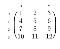
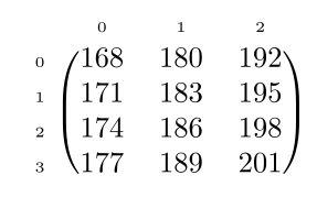
Consider the following matrix (with row labels 0-3 and column labels 0-2):

Row-Major Storage

List off all the elements of this matrix in the order that they are stored in memory: $[1, 2, 3, 4, 5, 6, 7, 8, 9, 10, 11, 12]$.

This output is due to the underlying assumption made by computer scientists that matrices are row-major: list off each element of a given row, and proceed row by row. If the above matrix is row-major, then its dimensions are $4 \times 3$.

Column-Major Storage

Mathematicians traditionally consider matrices in a column-major fashion: list off each element of a given column, and proceed column by column. Listing off all the elements of this matrix in order: $[1, 4, 7, 10, 2, 5, 8, 11, 3, 6, 9, 12]$.

If the matrix is column-major, then its dimensions are $3 \times 4$.

In fact, Excel exhibits column-major addressing as evidenced by the fact that a cell address in Excel lists a letter first (column) and then a number (row). (Note: One would have to check how Excel internally stores and accesses the worksheet, but externally it does appear to be column-major.)

Accessing Elements: Row-Major

Even accessing just one 2D cell within the actual 1D storage will be different depending on whether you assume row-major or column-major.

What is the value of $\text{Matrix}[1,2]$?

If the matrix is accessed in a row-major fashion, then $\text{Matrix}[1,2] = 6$.

If the matrix is accessed in a column-major fashion, then $\text{Matrix}[1,2] = 8$.

As mentioned above, computer scientists assume row-major unless explicitly stated otherwise.

Memory Address Formulas

For simplicity of this discussion, assume that each cell of the matrix only requires one memory address per cell location. Then, a matrix of size $m \times n$ requires $m \cdot n$ memory addresses, which we will index from $0$ to $(mn - 1)$.

In most programming languages, the name of the array (here, simply Matrix) contains the base (first) address of the array so that the Matrix address is the memory location of $\text{Matrix}[0,0]$.

Row-Major Address Formula

$$\text{Matrix}[i,j] = \text{Address}(\text{Matrix}) + (i \cdot n) + j$$

Column-Major Address Formula

$$\text{Matrix}[i,j] = \text{Address}(\text{Matrix}) + (i \cdot m) + j$$

Example: Memory Address Calculation

Consider the above matrix and assume that Matrix is at location 168. (This would never actually occur because the first million addresses or so are strictly guarded and reserved for the operating system code running the computer, called the kernel. But to keep our arithmetic simple, let us assume the first address is 168 and that the contents of each cell only requires one address.)

Then, the actual addresses in memory are as follows (row-major):

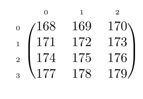
Apply the formula to location $\text{Matrix}[2,1]$ (row index 2, column index 1):

For row major:

$$\text{Matrix}[i,j] = \text{Address}(\text{Matrix}) + (i \cdot n) + j$$

Given:

• $m = 4$ (rows)
• $n = 3$ (columns)
• $i = 2$ (row position)
• $j = 1$ (column position)
• $\text{Address}(\text{Matrix}) = 168$ (base address)

$$\text{Matrix}[2,1] = 168 + (2 \cdot 3) + 1 = 168 + 6 + 1 = 175$$

Column-Major Address Example

If the matrix is stored in column-major format, the addresses would be located as follows:

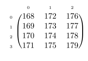
Using the column-major formula:

$$\text{Matrix}[i,j] = \text{Address}(\text{Matrix}) + (i \cdot m) + j$$ $$\text{Matrix}[2,1] = 168 + (2 \cdot 4) + 1 = 168 + 8 + 1 = 177$$

Multi-Byte Data Types

If each cell of the matrix requires data_type number of bytes (e.g., for a matrix of objects), then the starting addresses of each matrix cell have to be adjusted.

Row-Major with Multi-Byte Data Types

$$\text{Matrix}[i,j] = \text{Address}(\text{Matrix}) + (i \cdot n + j) \cdot \text{data\_type}$$

Example: Suppose each matrix cell requires 3 memory locations (bytes). Then, the starting addresses for each cell location are:

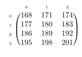
For $\text{Matrix}[2,1]$:

• $m = 4$ (rows)
• $n = 3$ (columns)
• $i = 2$ (row position)
• $j = 1$ (column position)
• $\text{Address}(\text{Matrix}) = 168$ (base address)
• $\text{data\_type} = 3$ (length of data type)

$$\text{Matrix}[2,1] = 168 + (2 \cdot 3 + 1) \cdot 3 = 168 + 7 \cdot 3 = 168 + 21 = 189$$

The cell occupies addresses 189, 190, and 191.

Column-Major with Multi-Byte Data Types

$$\text{Matrix}[i,j] = \text{Address}(\text{Matrix}) + (i \cdot m + j) \cdot \text{data\_type}$$

For the same matrix with 3 bytes per cell:

For $\text{Matrix}[2,1]$:

$$\text{Matrix}[2,1] = 168 + (2 \cdot 4 + 1) \cdot 3 = 168 + 9 \cdot 3 = 168 + 27 = 195$$

The cell occupies 3 bytes: addresses 195, 196, and 197.

Notation: Matrix[i,j] vs. Matrix[i][j]

Mathematical notation uses $\text{Matrix}[i,j]$ to refer to matrix cells, but Java uses $\text{Matrix}[i][j]$ notation instead. Some programming languages allow for either notation. Is there an inherent difference between the two notations?

Yes! But you need to read a specific programming language manual as to whether this distinction is actually implemented. In the case of Java, it would seem that this distinction is made, and Java does not support the inherent meaning of $\text{Matrix}[i,j]$ but only of $\text{Matrix}[i][j]$.

Matrix[i,j]: Contiguous Storage

The notation $\text{Matrix}[i,j]$ signifies that all the cells of the matrix are stored sequentially in one contiguous memory range of locations. Thus, the formulas discussed above hold true.

Matrix[i][j]: Array of Arrays

The notation $\text{Matrix}[i][j]$ signifies $\text{Matrix}[]$ of $[]$, meaning a 1D array each cell of which is pointing to a separate 1D array (an array of lists in the first dimension).

For row-major, $\text{Matrix}[4][3]$ would be stored such that:

Row-Major Example:

The key point here is that each row can be independently stored in very different areas of memory. The starting address location for each of these rows is stored in the header 1D structure for this simulated 2D matrix.

A similar discussion can be made for column-major, but especially here, this is more about perception than reality of storage.

Column-Major Example:

Higher Dimensions

The Java perspective of a 3D matrix $\text{Matrix3D}[][][]$ would similarly be a 1D array of 1D arrays, each pointing to a (third) 1D array containing the data. And so on for higher dimensions.

If, however, these higher-dimensional arrays are implemented in contiguous memory, then updated formulas involving all dimensional sizes would have to be formulated.

Trees

Storing Trees in Linear Memory

The question we are dealing with is: if the Turing machine tape were endowed with RAM properties using 1D memory, how can multidimensional structures be stored on the tape?

The previous section dealt with arrays and matrices. This section deals with graphs and trees.

Trees vs. Adjacency Matrices

Graphs can technically be stored in adjacency matrices, which is covered by the previous section’s discussion. Technically, a tree is a graph, so it can also be covered by the previous section’s discussion on matrices and arrays, but not in an efficient manner.

Since trees with $n$ nodes can only have $n-1$ edges, and the adjacency matrix stores up to $n^2$ edges, which for trees will mostly contain zeros (since most of those potential edges will not exist), this is a sparse matrix. In mathematics, a sparse matrix is when the actual data $\ll$ storage cells for the data (here, $n-1$ vs. $n^2$).

This section discusses a much more efficient mapping of trees to RAM, or 1D arrays.

Binary Tree Array Mapping

Consider a binary tree structure:

Tree Traversal Methods

There are a number of ways to traverse or explore data stored in a tree:

• Inorder, Preorder, Postorder Traversals
• Breadth-First Search (BFS)
• Depth-First Search (DFS)

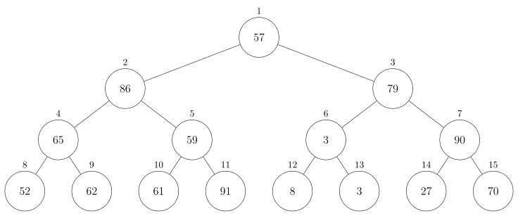
The “data” in the cells of the above tree numbers the nodes in a breadth-first search (BFS) manner (i.e., level by level).

Thus, the BFS for the above tree is: $[57, 86, 79, 65, 59, 3, 90, 52, 62, 61, 91, 8, 3, 27, 70]$.

Binary Encoding of Paths

Traditionally, when traversing trees, we talk about Left (L) and Right (R) movements.

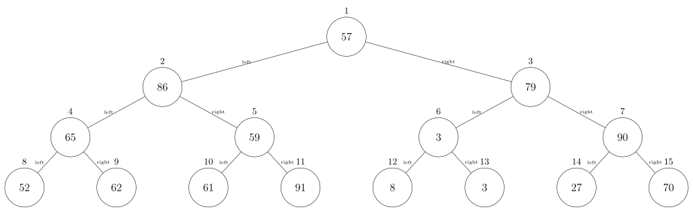
For example, to traverse from the root to node 11, you would go Left, Right, Right (LRR).

Using Binary Representation

Let us consider the exact same configuration but assign 0 to Left and 1 to Right. We will consider entering the tree as going “Right” to the Root, and if we go “Left” and did not get to the Root, we consider this as an “Empty” tree.

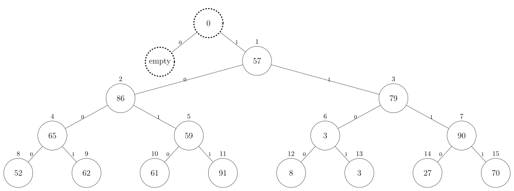
The tree contains 15 nodes, indexed from 1 to 15:

Index	Node	Binary Index	Directions
1	57 (root)	1	R
2	86	10	RL
3	79	11	RR
4	65	100	RLL
5	59	101	RLR
6	3	110	RRL
7	90	111	RRR
8	52	1000	RLLL
9	62	1001	RLLR
10	61	1010	RLRL
11	91	1011	RLRR
12	8	1100	RRLL
13	3	1101	RRRL
14	27	1110	RRRL
15	70	1111	RRRR

Key Insight: The binary of the indices encodes the pathway of getting to the tree and traversing to the node of interest. The length of this binary is the level number. This is an efficient storage mechanism for the two-dimensional tree into a 1D array such as the Turing machine tape.

Finding Parent and Child Nodes

The follow-up question is: from a given node, how do we determine the children and parent nodes?

If we had a two-dimensional structure, we could basically do that, but what about this 1D storage simulation?

The following approach automatically has the parent index information without requiring us to do anything extra for it. (Note: Our classic programming approach to tree nodes does not have a field for parent. It is only the iterative or recursive nature of usage that maintains who is the parent.)

Finding the Parent Node

Consider Node 5, which in binary is 101. It is not by accident that its parent is Node 2, which in binary is 10 (simply shift the binary right by one bit).

Consider Node 9, which in binary is 1001. It is not by accident that its parent is Node 4, which in binary is 100 (simply shift the binary right by one bit).

This determines the parent node. Mathematically, this is the same as integer division (ignore fractional remainder) of the index number by 2.

$$\text{Parent index} = \lfloor \text{node index} / 2 \rfloor$$

Finding the Child Nodes

Consider Node 5, which in binary is 101. It is not by accident that its children are 101(0) and 101(1), or nodes 10 and 11.

Consider Node 3, which in binary is 11. It is not by accident that its children are 11(0) and 11(1), or nodes 6 and 7.

This determines the children nodes. Mathematically:

$$\text{Left child index} = \text{node index} \times 2$$ $$\text{Right child index} = (\text{node index} \times 2) + 1$$

Connection to Heapsort

This observation is inherent in the heapsort algorithm.

The original version actually stored the data in a tree data structure with nodes. Subsequently (later that year), it was realized that it could be simulated by an array in a similar manner as described above.

• John William Joseph Williams (1964) used a tree structure
• R. W. Floyd (1964) used an array