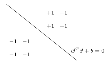
Given a linearly separable dataset D, our goal is to find the w and b which creates the hyperplane with maximum margin.
To do so, we must solve the following optimization:
w,bargmaxγ(w,b)
subject to
∀i,yi(wTxi+b)≥0
Without this constraint, the hyperplane would simply fly off to infinity — the margin can be made arbitrarily large just by moving the hyperplane infinitely far away from all the data. The constraint is what keeps it properly anchored over the dataset.
This is equivalent to:
w,bargminwTw
subject to:
∀i,yi(wTxi+b)≥0
minxi∈DwTxi+b=1
Which is further equivalent to:
w,bargminwTw
subject to
∀i,yi(wTxi+b)≥1
The condition ∀i,yi(wTxi+b)>0 serves two purposes: it ensures the hyperplane correctly classifies all points, and it keeps the hyperplane from flying off to infinity. That is, it ensures we get something like this:
For all positive points, since minxi∈DwTxi+b=1:
⇒∀i,wTxi+b≥1
And since yi=1:
⇒yi(wTxi+b)≥1
For all negative labels, since minxi∈DwTxi+b=1:
⇒∀i,wTxi+b≤−1
And since yi=−1:
⇒∀i,yi(wTxi+b)≥1
This is the same constraint as for positive yi‘s.
We now have the answer to how to find the w and b that maximizes the margin in a linearly separable dataset.
The points that sit exactly on one of the two margin boundaries — satisfying yi(wTxi+b)=1 with equality — are called support vectors. They are the only points that determine the position and orientation of the hyperplane; every other correctly classified point could be removed from the dataset and the solution would be unchanged. This is where the name “Support Vector Machine” comes from.
The reason we spent all that time transforming the original problem into this QP form is practical: early ML researchers couldn’t solve the original max-margin formulation directly. Mathematicians, however, had already been studying quadratic programming for years and had well-developed tools for it. Reformulating as a QP opened the door to those existing solutions.
There are several approaches to solving QP problems:
Active set methods (1950s/60s)
Interior point methods (1980s)
Subgradient method (1960s/70s) — we are studying this
The subgradient method is closely related to the gradient descent we’ve already studied — think of it as gradient descent with an extra constraint-checking step. It is somewhat outdated (SMO is today’s standard), but it works and is much easier to understand without a full course in numerical analysis.
To solve the optimization, we:
Initialize — choose values for w, b, α
For each datapoint (xi,yi), check if the constraint is satisfied: is yi(wTxi+b)≥1?
Yes:
wnew=wold−αwold
bnew=bold
No:
wnew=wold−α(wold−yixi)
bnew=bold+αyi
Repeat until convergence — that is, until the constraints are always satisfied and w and b stop meaningfully changing between updates.
This completes phase 3.
Phase 4: Modifying the Approach for the Original Problem
Original problem: Given a dataset which is not linearly separable, find the hyperplane which maximizes the margin.
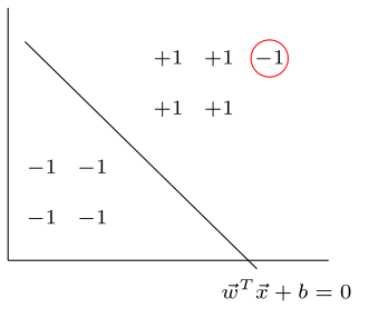
In the case the data is NOT linearly separable, no such hyperplane will satisfy the condition:
∀i,yi(wTxi+b)≥1
For the misclassified point, wTxi+b has the wrong sign relative to yi, so:
yi(wTxi+b)<0
But it needs to be yi(wTxi+b)≥1.
Idea: Relax the condition/constraint by softening it. This gives leeway, and produces the “SVM with soft margins” (also called “SVM with slack variables”).
The intuition is that in the case where the dataset is not linearly separable, we aim to satisfy:
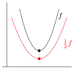
w,bargmin21wTwsubject to∀i,yi(wTxi+b)≥1
as much as possible, but will allow some violation by adding a little slack ξ.
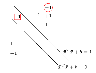
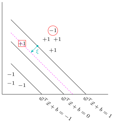
Consider this data:
For the red-boxed +1 point, wTxi+b<1. Since yi=1:
⇒yi(wTxi+b)<1⇒∀i,yi(wTxi+b)≥1 is violated
Let’s say wTxi+b=0.4. Although this condition is not satisfied, we will satisfy:
yi(wTxi+b)≥1−ξas long as ξ≥0.6
For the red-circled −1 point (misclassified, past the positive margin boundary), wTxi+b>1. Since yi=−1, and multiplying a positive number by −1 flips the sign:
⇒yi(wTxi+b)<−1(condition is violated)
For example, yi(wTxi+b)=−3. Again, we introduce slack — this point will satisfy: