Lec 05-07-2026: Support Vector Machines: Maximizing the Margin

Recall

Given a linearly separable dataset $D$ , our goal is to find the hyperplane $\vec{w}^T \vec{x} + b = 0$ which maximizes the margin — the distance from the hyperplane to the closest point.

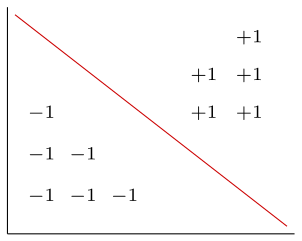
$Linearly separable graph: Scatter plot with -1 points in the lower-left and +1 points in the upper-right, separated by a red diagonal hyperplane$

The distance from a point to the hyperplane is given by:

\frac{|\vec{w}^T \vec{x} + b|}{\|\vec{w}\|}

The Margin

\underbrace{\gamma(\vec{w}, b)}_{\text{the margin}} := \min_{\vec{x}_i \in D} \frac{|\vec{w}^T \vec{x}_i + b|}{\|\vec{w}\|}

$Flow diagram: hyperplane (w,b) maps to gamma, which gives the distance to the closest point (the margin)$

Think of $\gamma$ as a machine: you feed it a hyperplane by specifying $\vec{w}$ and $b$ , and it returns a single number — the distance to the closest data point. That number is the margin for that particular hyperplane. Different hyperplanes give different margin values.

Maximizing the Margin

We must consider all possible hyperplanes. For instance, on a given dataset, one hyperplane may give a margin of 1.1 (distance to the closest point, circled):

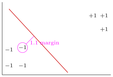
$Scatter plot with a red hyperplane positioned close to the -1 cluster; the nearest -1 point is circled with a perpendicular line to the hyperplane labeled 1.1 margin$

Since our goal is to maximize the margin, we must find:

\underset{\vec{w},\, b}{\arg\max}\; \gamma(\vec{w}, b)

where $\arg\max_{\vec{w}, b}$ denotes the inputs $\vec{w}, b$ that achieve the maximum. For example:

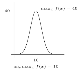
$Bell curve f(x) peaking at x=10 with max value 40, showing max f(x)=40 and argmax f(x)=10$

Here, the subscript $x$ in $\max_x$ and $\arg\max_x$ means “over all $x$ ” - i.e., we range over every possible value of $x$ to find the maximum and the input that achieves it.

Concretely: fix one $(\vec{w}, b)$ , compute all point-to-hyperplane distances, take the minimum — that is $\gamma$ for that hyperplane. Try a different $(\vec{w}, b)$ , repeat. After doing this across all hyperplanes, you end up with a collection of margins — say $1,\; 1.1,\; 1.6, \ldots$ — and return the $\vec{w}$ and $b$ that produced the largest one.

Small Hiccup

If our only goal is to maximize the margin, we run into a problem:

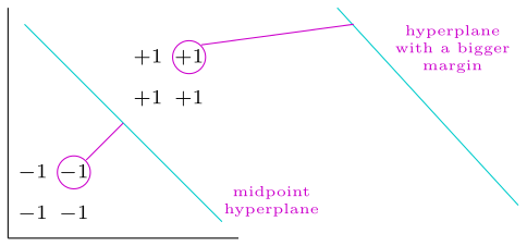
$Two panels: left shows midpoint hyperplane separating -1 cluster (lower-left, one circled) and +1 cluster (upper-right, one circled); right shows a larger-margin hyperplane far from the data$

The computer, in attempting to maximize the margin (i.e. to maximize the distance from the hyperplane to the nearest point), will send the hyperplane to infinity — this is bad because we want the hyperplane to separate the two classes.

Fixing the Hiccup

Q: How do we fix this?

A: Impose a constraint which tells the computer to make sure the hyperplane separates the two classes.

To see what form this constraint should take, recall that $y_i \in \{-1, +1\}$ is the label of point $\vec{x}_i$ , and that $\vec{w}^T \vec{x}_i + b$ is the signed output of the hyperplane at $\vec{x}_i$ — it is positive on one side of the hyperplane and negative on the other. If a point is on the correct side of the hyperplane for its class, then $y_i$ and $\vec{w}^T \vec{x}_i + b$ have the same sign, so their product is positive. If the point is on the wrong side, the signs are opposite and the product is negative.

So requiring:

\forall i,\; y_i \left(\vec{w}^T \vec{x}_i + b\right) \geq 0

is a compact way of saying “every data point must be on the correct side of the hyperplane.” Two things still need to be verified:

Does this actually force the hyperplane to lie between the two classes?
Does this prevent the hyperplane from flying off to infinity?

Here is Why

Updated goal:

\underset{\vec{w},\, b}{\arg\max}\; \gamma(\vec{w}, b) \quad \text{subject to} \quad y_i(\vec{w}^T \vec{x}_i + b) \geq 0

Why It Solves the Problem

$Scatter plot: -1 cluster lower-left, +1 cluster upper-middle with one boxed +1 on the wrong side; blue hyperplane labeled w^T x+b=0 is far right, and a magenta pointer connects the boxed +1 to the hyperplane$

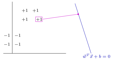
For this datapoint $x_i$ (labeled $y_i = +1$ , but on the wrong side of the hyperplane), it must be the case that $\vec{w}^T \vec{x}_i + b < 0$ :

\begin{aligned} &\Rightarrow 1 \cdot (\vec{w}^T \vec{x}_i + b) < 0 \quad \text{(multiply by } y_i = 1\text{)} \\ &\Rightarrow y_i(\vec{w}^T \vec{x}_i + b) < 0 \end{aligned}

This violates the constraint, so the hyperplane is forced to separate the two classes.

$Axes with horizontal line y=5; magenta-hatched region above labeled y>5; blue-hatched region below labeled y<5$

$Axes with diagonal hyperplane w^T x+b=0; triangular region between axes and hyperplane is blue-hatched and labeled w^T x+b < 0$

Preventing the Hyperplane from Flying Off to $-\infty$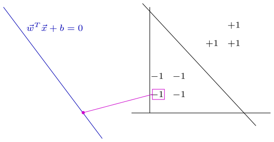

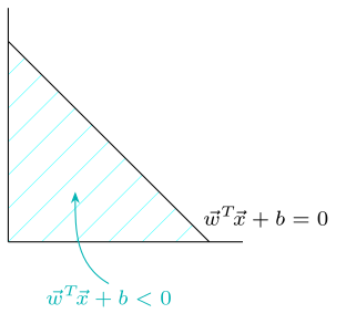
$Scatter plot: axes on the right with -1 cluster (one boxed) and +1 cluster; blue hyperplane labeled w^T x+b=0 has flown far left; magenta pointer connects boxed -1 to the hyperplane$

For this datapoint $x_i$ with label $y_i = -1$ : since it rests above the hyperplane, $\vec{w}^T \vec{x}_i + b > 0$ :

\begin{aligned} &\Rightarrow (-1)(\vec{w}^T \vec{x}_i + b) < 0 \\ &\Rightarrow y_i(\vec{w}^T \vec{x}_i + b) < 0 \end{aligned}

The constraint is again violated, so the hyperplane cannot fly off to $-\infty$ .

One Final Comment on This Constraint

This constraint allows for the midpoint hyperplane to be considered, allowing us to place the hyperplane in between the 2 classes, which is what we want.

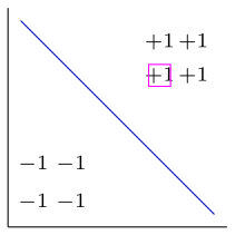
$Scatter plot with the midpoint hyperplane correctly separating the clusters; the +1 point closest to the hyperplane is boxed, showing it is above the hyperplane$

For this datapoint $x_i$ (labeled $y_i = +1$ , correctly above the hyperplane): $\vec{w}^T \vec{x}_i + b > 0$ :

\begin{aligned} &\Rightarrow 1 \cdot (\vec{w}^T \vec{x}_i + b) > 0 \\ &\Rightarrow y_i(\vec{w}^T \vec{x}_i + b) > 0 \end{aligned}

The constraint is satisfied.

Similarly, for a -1 point $x_j$ correctly below the hyperplane, $\vec{w}^T \vec{x} + b < 0$ :

$Scatter plot with the midpoint hyperplane correctly separating the clusters; the -1 point closest to the hyperplane is boxed, showing it is below/left of the hyperplane$

\begin{aligned} &\Rightarrow (-1)(\vec{w}^T \vec{x} + b) > 0 \\ &\Rightarrow y_i(\vec{w}^T \vec{x} + b) > 0 \end{aligned}

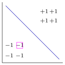
Hence, the condition is satisfied: $\forall i,\; y_i(\vec{w}^T \vec{x}_i + b) \geq 0$ places the hyperplane where it is wanted.

Constrained Optimization

\underset{\vec{w},\, b}{\arg\max}\; \gamma(\vec{w}, b) \quad \text{subject to} \quad y_i(\vec{w}^T \vec{x}_i + b) \geq 0

is a constrained optimization problem. In a constrained optimization problem, we are not free to search over all possible values of our variables — we can only consider values that satisfy the constraint. Think of it as finding the best solution within a restricted set: instead of a global maximum, we find the best answer among the options the constraint allows.

A familiar example from calculus illustrates the idea:

Example from Calculus

$Rectangle with top side on a river (no fence needed), left side labeled x, bottom labeled y$

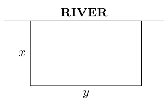
Q: Find the area of the maximum rectangular garden given the farmer only has 1000ft of fencing.

\Rightarrow \text{Goal: } \underset{x,\, y}{\arg\max}\; \text{Area} \quad \text{subject to} \quad 2x + y = 1000

Rewriting the Optimization Problem

We want to simplify this into a form that is easier to work with. Start by substituting the definition of $\gamma$ :

\underset{\vec{w},\, b}{\arg\max}\; \gamma(\vec{w}, b) = \underset{\vec{w},\, b}{\arg\max}\; \min_{\vec{x}_i \in D} \frac{|\vec{w}^T \vec{x}_i + b|}{\|\vec{w}\|}

The min is taken over all data points $\vec{x}_i$ . The denominator $\|\vec{w}\|$ doesn’t depend on $\vec{x}_i$ — once you fix a hyperplane, $\|\vec{w}\|$ is just a constant — so it can be factored out:

= \underset{\vec{w},\, b}{\arg\max}\; \frac{1}{\|\vec{w}\|} \min_{\vec{x}_i \in D} |\vec{w}^T \vec{x}_i + b|

The Scaling Trick

Here is a key observation from algebra: the line $y = 2x + 5$ and the line $7y = 14x + 35$ are the same geometric line — multiplying both sides by 7 doesn’t change it. The same applies to hyperplanes: you can scale $(\vec{w}, b)$ by any non-zero constant and it still describes the same hyperplane.

Since we are searching over all possible hyperplanes anyway, we are free to choose how we write any given hyperplane. We will use this freedom to always normalize $(\vec{w}, b)$ so that the minimum numerator equals 1:

\min_{\vec{x}_i \in D} |\vec{w}^T \vec{x}_i + b| = 1

To see why this is always possible: suppose you have some $(\vec{w}, b)$ and the minimum comes out to 15. Replace $\vec{w}$ with $\vec{w}/15$ and $b$ with $b/15$ — this still describes the same hyperplane, but now the minimum is $15/15 = 1$ . You can always rescale to make the minimum 1, so this isn’t an extra restriction — it’s just a choice of normalization.

With the minimum fixed at 1, it drops out and the problem simplifies to:

\underset{\vec{w},\, b}{\arg\max}\; \frac{1}{\|\vec{w}\|}

Turning Maximization into Minimization

$\|\vec{w}\|$ is a positive scalar. To maximize $\frac{1}{\|\vec{w}\|}$ , think about how $\frac{1}{x}$ behaves: as $x$ gets smaller, $\frac{1}{x}$ gets larger. So the maximum of $\frac{1}{\|\vec{w}\|}$ occurs exactly when $\|\vec{w}\|$ is as small as possible. Maximizing $\frac{1}{\|\vec{w}\|}$ and minimizing $\|\vec{w}\|$ have the same solution:

\underset{\vec{w},\, b}{\arg\max}\; \frac{1}{\|\vec{w}\|} = \underset{\vec{w},\, b}{\arg\min}\; \|\vec{w}\| = \underset{\vec{w},\, b}{\arg\min}\; \sqrt{\vec{w}^T \vec{w}}

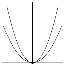
Removing the Square Root

Minimizing $\sqrt{\vec{w}^T \vec{w}}$ and minimizing $\vec{w}^T \vec{w}$ produce the same argmin. Squaring is a monotone transformation for non-negative values — if $a < b$ then $a^2 < b^2$ — so it preserves which value is smallest. Wherever $\|\vec{w}\|$ is minimized, $\|\vec{w}\|^2 = \vec{w}^T \vec{w}$ is minimized there too. This is the same idea used in calculus when minimizing distances: rather than minimizing $d = \sqrt{(x_2-x_1)^2 + (y_2-y_1)^2}$ , you minimize $d^2 = (x_2-x_1)^2 + (y_2-y_1)^2$ instead, which avoids dealing with the square root.

$Two parabolas of different widths sharing the same minimum point, illustrating that squaring a function does not change the argmin$

= \underset{\vec{w},\, b}{\arg\min}\; \vec{w}^T \vec{w}

The square root is gone, which makes this much cleaner to work with. To be precise: the constraint didn’t disappear during the rewriting above — only the objective was being simplified. The full problem, with the constraint restored, is:

\underset{\vec{w},\, b}{\arg\min}\; \vec{w}^T \vec{w} \quad \text{subject to} \quad y_i(\vec{w}^T \vec{x}_i + b) \geq 0 \;\; \forall i

This is the standard form of the SVM optimization problem: minimize a quadratic objective subject to linear constraints. Problems of this form have well-developed solution techniques, which is what comes next.