Lec 04-14-2026: Coordinates and Vectors | MATH 245
Road Map
Section titled “Road Map”- Unit 1 - Intro to modeling & G.D.
- Unit 2 - Overview of neural networks
- Unit 3 - Linear Algebra & Support Vector Machines
- Unit 4 - Recommendation Algorithm Overview
- Unit 5 - Simple financial models
Throughout this course, we’ve posed some meaningful questions:
-
- How does a machine learn?
- How can we find the minimum of a cost function?
- How does text recognition work?
- How can an image be made numeric?
- Can we simplify the notation for a neural network?
- Can we improve our house price model? where = square feet
All of the above questions require us to work in a higher-dimensional space of real numbers, and this is a part of Linear Algebra! For us, in modeling, we often observe a phenomenon and the drivers/causes of this phenomenon requires higher dimensions.
To progress any further, we’ll need a crash-course in elementary linear algebra.
Coordinates and Vectors
Section titled “Coordinates and Vectors”Coordinates: At first, we may attribute the idea of coordinates to the work in geometry by classic Greek mathematicians (600 BCE - 300 CE).
Geometry takes place in a flat 2D plane or 3D space.
- 2D plane: circles, rectangles
- 3D space: spheres
Amazingly enough, the idea of a coordinate system wasn’t introduced until René Descartes (French mathematician, 1637).
There’s this huge gap because for most of time, algebra & geometry were seen as different fields.
Using a coordinate system allows us to connect geometric objects, like lines, to algebraic objects like equations - a bridge between algebra and geometry that lets us study shapes using equations, and equations using geometry.
Ex.
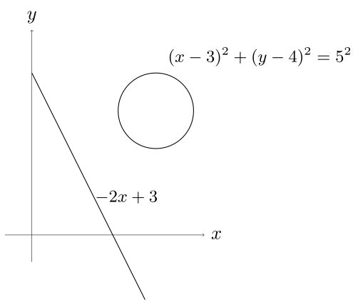
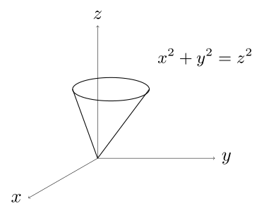
When we have 2D or 3D, we typically use the -plane of the -coordinate system.
For us, we’ll have many coordinates, so we’ll use the coordinate system.
Vectors
Section titled “Vectors”In the 2D plane, let’s consider the coordinate and draw an arrow from the origin to :
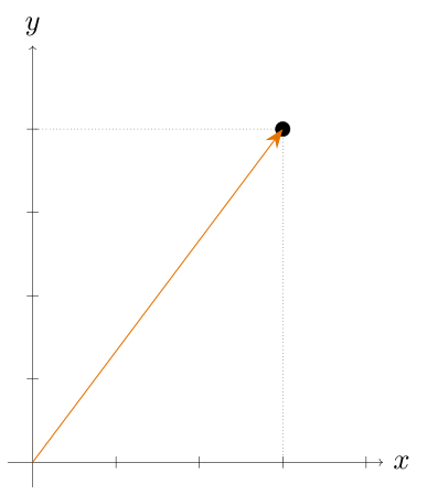
- This arrow is called a vector
- The origin is called its initial point
- The tip of the arrow is called its terminal point
How do we denote a vector? We write .
By default, we write vectors as column vectors (entries stacked vertically):
When we want to write a vector in a single row (as a row vector), we use the transpose notation, written :
The transpose simply “rotates” the vector from a column to a row (or vice versa). We’ll see the transpose come up often in later computations.
Notice as we change the terminal point, the direction & length change. For this reason, we say a vector is defined by its direction & length (also called its magnitude or norm). Its starting point does not matter.
Loosely speaking, there are 2 types of quantities in math:
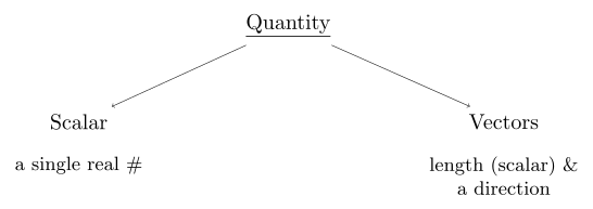
Scalar - a single real number
Ex. , meters
Vector - a length (scalar) & a direction
Ex. wind direction mph SE, displacement (physics)
Without a direction, it’s a scalar.
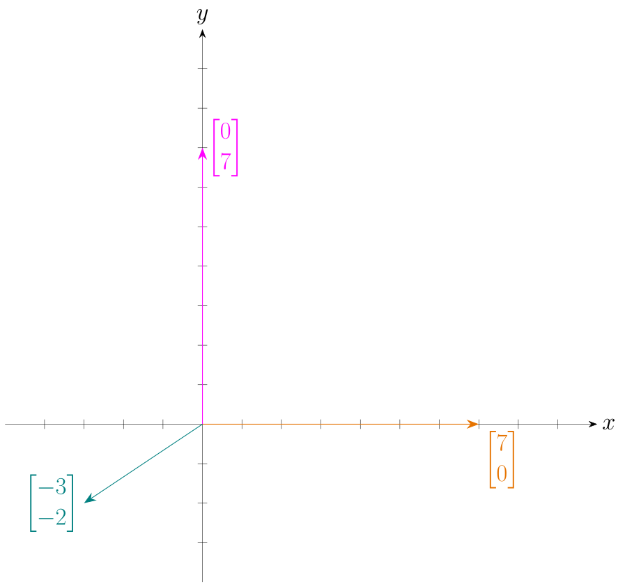
In , plot , , :
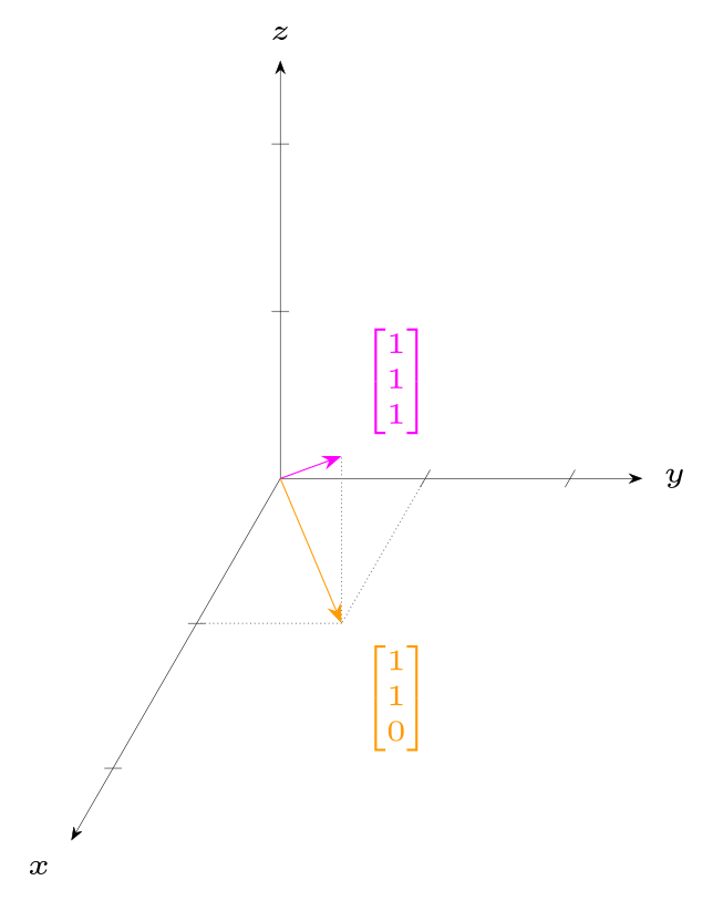
In , plot , :
Earlier we said vectors are completely characterized by their length & direction - their starting position does not matter.
As long as 2 vectors have the same length & direction, then these vectors are equal, regardless of where they are drawn.
Ex.
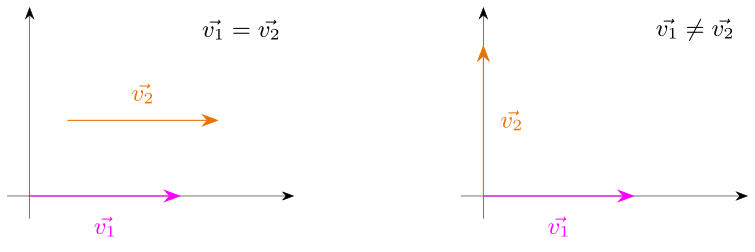
In the left diagram, and point in the same direction and have the same length - they are equal even though they start at different points. In the right diagram, they point in different directions, so they are not equal.
Two vectors are equal provided they are translations of each other (same direction, same length, just shifted).
For convenience, we’ll always make sure our vectors start at the origin. This way, a vector is completely characterized by its terminal point alone - no need to also track the starting point.
Def. The zero vector, denoted by , is the vector whose initial & terminal point are the same. It has length 0, and since it doesn’t point anywhere, its direction is undefined.
Mathematics follows a consistent pattern: first, we define a structure - a collection of objects we care about. Then we define an algebra on that structure, meaning a set of operations that let us combine and manipulate those objects. This pattern appears throughout all of mathematics:
| Structure | Algebra |
|---|---|
| numbers: | |
| functions: | (function compositions: ) |
| sets | |
| statements |
We’ll now define an algebra on vectors - starting with addition.
Vector Addition
Section titled “Vector Addition”The idea is simple: to add two vectors, just add their corresponding components.
Def. Given vectors & in , we define
That is, add the first components together, and add the second components together (component-wise addition). This extends naturally to higher dimensions - just add each pair of matching components:
Def. Given vectors & in , we define
Note: you can only add two vectors if they have the same number of components (same dimension).
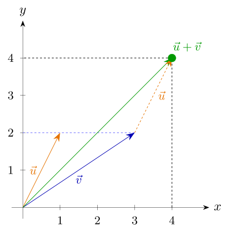
Ex (): If & , then
Two ways to geometrically consider this:
- In each direction, we add the components to get the total horizontal & total vertical displacement.
- Tail-to-Tip method: Slide so that its starting point sits on the tip of . The new arrow drawn from the origin to the tip of the repositioned is . Visually, the three vectors form a triangle.