Lec 05-14-2026: Soft-Margin SVM & Cross-Validation

Soft-Margin SVM

Last lecture, we started the soft-margin SVM. We said: given a non-linearly separable dataset $D$, to find the optimal hyperplane $\vec{w}^T \vec{x} + b = 0$ which maximizes the margin, we solve the following optimization problem:

$$\arg\min_{\vec{w}, b} \underbrace{\frac{1}{2} \vec{w}^T \vec{w}}_{\text{how large margin can be}} + \underbrace{C \sum_{i=1}^{n} \xi_i}_{\substack{\text{wants to make margin small} \\ \text{(penalizes constraint violations)}}}$$

Subject to $\forall i$, $y_i (\vec{w}^T \vec{x}_i + b) \geq 1 - \xi_i$ and $\forall i$, $\xi_i \geq 0$

Comments

Because $\xi_i$ is a measure of how much a point violates the margin, we wish to minimize the total violation, and that’s why we are minimizing $\sum_{i=1}^{n} \xi_i$.

• $\xi_i$ is a measure of how much datapoint $i$ measures the error.
• So $\sum \xi_i$ is a measure of the total violation of the margin across all datapoints.

$C \sum_{i=1}^{n} \xi_i$ is saying “I’ll allow some points to break the margin but charge a fee of $C$ units per violation.”

• If $C$ is low, it is cheap to break the margin, so we get a larger margin.
• If $C$ is high, it is expensive to break the margin, so the margin / breathing room will decrease to make sure there are fewer violations.

So we want to maximize the margin and minimize violations at the same time — $C$ is what controls that balance.

Cross-Validation for Selecting $C$

We split the data as follows:

Training Phase

Using the 60% training split, we train 5 models with different values of $C$:

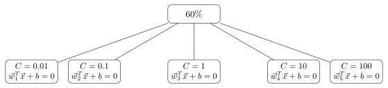
Which $C$ yields a better model?

We use each of the 5 models to predict on the validation data and compute the accuracy.

• Use the $C$ coming from the highest accuracy.

Using this $C$, run the optimization on the training + validation set. This yields $\vec{w}_\text{final}$ and $b_\text{final}$, and our end model is $\vec{w}_\text{final}^T \vec{x} + b_\text{final} = 0$.

We use our end model on the test set, which the model has never seen before, so we get an “honest” reading.