In our last lecture, we applied the Law of Cosines to vector subtraction in order to motivate the notion of the dot product.
If u ⃗ , v ⃗ ∈ R n \vec{u}, \vec{v} \in \mathbb{R}^n u , v ∈ R n u ⃗ = [ u 1 u 2 ⋮ u n ] \vec{u} = \begin{bmatrix} u_1 \\ u_2 \\ \vdots \\ u_n \end{bmatrix} u = u 1 u 2 ⋮ u n v ⃗ = [ v 1 v 2 ⋮ v n ] \vec{v} = \begin{bmatrix} v_1 \\ v_2 \\ \vdots \\ v_n \end{bmatrix} v = v 1 v 2 ⋮ v n
u ⃗ T v ⃗ = [ u 1 u 2 ⋯ u n ] [ v 1 v 2 ⋮ v n ] : = u 1 v 1 + u 2 v 2 + ⋯ + u n v n \vec{u}^T\vec{v} = \begin{bmatrix} u_1 & u_2 & \cdots & u_n \end{bmatrix} \begin{bmatrix} v_1 \\ v_2 \\ \vdots \\ v_n \end{bmatrix} := u_1v_1 + u_2v_2 + \cdots + u_nv_n u T v = [ u 1 u 2 ⋯ u n ] v 1 v 2 ⋮ v n := u 1 v 1 + u 2 v 2 + ⋯ + u n v n Additionally, from two lectures ago, we said:
If w ⃗ = [ w 1 w 2 ⋮ w n ] ∈ R n \vec{w} = \begin{bmatrix} w_1 \\ w_2 \\ \vdots \\ w_n \end{bmatrix} \in \mathbb{R}^n w = w 1 w 2 ⋮ w n ∈ R n ∥ w ⃗ ∥ = w 1 2 + w 2 2 + ⋯ + w n 2 \|\vec{w}\| = \sqrt{w_1^2 + w_2^2 + \cdots + w_n^2} ∥ w ∥ = w 1 2 + w 2 2 + ⋯ + w n 2 ∥ w ⃗ ∥ 2 = w 1 2 + w 2 2 + ⋯ + w n 2 \|\vec{w}\|^2 = w_1^2 + w_2^2 + \cdots + w_n^2 ∥ w ∥ 2 = w 1 2 + w 2 2 + ⋯ + w n 2
Notice:
w ⃗ T w ⃗ = [ w 1 w 2 ⋯ w n ] [ w 1 w 2 ⋮ w n ] = w 1 2 + w 2 2 + ⋯ + w n 2 \vec{w}^T\vec{w} = \begin{bmatrix} w_1 & w_2 & \cdots & w_n \end{bmatrix} \begin{bmatrix} w_1 \\ w_2 \\ \vdots \\ w_n \end{bmatrix} = w_1^2 + w_2^2 + \cdots + w_n^2 w T w = [ w 1 w 2 ⋯ w n ] w 1 w 2 ⋮ w n = w 1 2 + w 2 2 + ⋯ + w n 2 Hence ∥ w ⃗ ∥ 2 = w ⃗ T w ⃗ \|\vec{w}\|^2 = \vec{w}^T\vec{w} ∥ w ∥ 2 = w T w ∥ w ⃗ ∥ = w ⃗ T w ⃗ \|\vec{w}\| = \sqrt{\vec{w}^T\vec{w}} ∥ w ∥ = w T w
u ⃗ T ( v ⃗ + w ⃗ ) = u ⃗ T v ⃗ + u ⃗ T w ⃗ \vec{u}^T(\vec{v} + \vec{w}) = \vec{u}^T\vec{v} + \vec{u}^T\vec{w} u T ( v + w ) = u T v + u T w 0 ⃗ T w ⃗ = 0 \vec{0}^T\vec{w} = 0 0 T w = 0 w ⃗ T v ⃗ = v ⃗ T w ⃗ \vec{w}^T\vec{v} = \vec{v}^T\vec{w} w T v = v T w ( c u ⃗ ) T v ⃗ = c ( u ⃗ T v ⃗ ) = u ⃗ T ( c v ⃗ ) (c\vec{u})^T\vec{v} = c(\vec{u}^T\vec{v}) = \vec{u}^T(c\vec{v}) ( c u ) T v = c ( u T v ) = u T ( c v ) u ⃗ \vec{u} u c c c ( c w ⃗ ) T = c w ⃗ T (c\vec{w})^T = c\vec{w}^T ( c w ) T = c w T
Justification of Property 1
LHS = u ⃗ T ( v ⃗ + w ⃗ ) = \vec{u}^T(\vec{v} + \vec{w}) = u T ( v + w )
u ⃗ T ( v ⃗ + w ⃗ ) = [ u 1 u 2 ⋯ u n ] ( [ v 1 v 2 ⋮ v n ] + [ w 1 w 2 ⋮ w n ] ) = [ u 1 u 2 ⋯ u n ] [ v 1 + w 1 v 2 + w 2 ⋮ v n + w n ] = u 1 ( v 1 + w 1 ) + u 2 ( v 2 + w 2 ) + ⋯ + u n ( v n + w n ) \begin{align*}
\vec{u}^T(\vec{v} + \vec{w})
&= \begin{bmatrix} u_1 & u_2 & \cdots & u_n \end{bmatrix}
\left(
\begin{bmatrix} v_1 \\ v_2 \\ \vdots \\ v_n \end{bmatrix}
+
\begin{bmatrix} w_1 \\ w_2 \\ \vdots \\ w_n \end{bmatrix}
\right) \\
&= \begin{bmatrix} u_1 & u_2 & \cdots & u_n \end{bmatrix}
\begin{bmatrix} v_1 + w_1 \\ v_2 + w_2 \\ \vdots \\ v_n + w_n \end{bmatrix} \\
&= u_1(v_1 + w_1) + u_2(v_2 + w_2) + \cdots + u_n(v_n + w_n)
\end{align*} u T ( v + w ) = [ u 1 u 2 ⋯ u n ] v 1 v 2 ⋮ v n + w 1 w 2 ⋮ w n = [ u 1 u 2 ⋯ u n ] v 1 + w 1 v 2 + w 2 ⋮ v n + w n = u 1 ( v 1 + w 1 ) + u 2 ( v 2 + w 2 ) + ⋯ + u n ( v n + w n ) RHS = u ⃗ T v ⃗ + u ⃗ T w ⃗ = \vec{u}^T\vec{v} + \vec{u}^T\vec{w} = u T v + u T w
u ⃗ T v ⃗ + u ⃗ T w ⃗ = [ u 1 u 2 ⋯ u n ] [ v 1 v 2 ⋮ v n ] + [ u 1 u 2 ⋯ u n ] [ w 1 w 2 ⋮ w n ] = u 1 v 1 + u 2 v 2 + ⋯ + u n v n + u 1 w 1 + u 2 w 2 + ⋯ + u n w n = u 1 v 1 + u 1 w 1 + u 2 v 2 + u 2 w 2 + ⋯ + u n v n + u n w n = u 1 ( v 1 + w 1 ) + u 2 ( v 2 + w 2 ) + ⋯ + u n ( v n + w n ) = LHS \begin{align*}
\vec{u}^T\vec{v} + \vec{u}^T\vec{w}
&= \begin{bmatrix} u_1 & u_2 & \cdots & u_n \end{bmatrix}
\begin{bmatrix} v_1 \\ v_2 \\ \vdots \\ v_n \end{bmatrix}
+
\begin{bmatrix} u_1 & u_2 & \cdots & u_n \end{bmatrix}
\begin{bmatrix} w_1 \\ w_2 \\ \vdots \\ w_n \end{bmatrix} \\
&= u_1v_1 + u_2v_2 + \cdots + u_nv_n
+ u_1w_1 + u_2w_2 + \cdots + u_nw_n \\
&= u_1v_1 + u_1w_1 + u_2v_2 + u_2w_2 + \cdots + u_nv_n + u_nw_n \\
&= u_1(v_1 + w_1) + u_2(v_2 + w_2) + \cdots + u_n(v_n + w_n) = \text{LHS}
\end{align*} u T v + u T w = [ u 1 u 2 ⋯ u n ] v 1 v 2 ⋮ v n + [ u 1 u 2 ⋯ u n ] w 1 w 2 ⋮ w n = u 1 v 1 + u 2 v 2 + ⋯ + u n v n + u 1 w 1 + u 2 w 2 + ⋯ + u n w n = u 1 v 1 + u 1 w 1 + u 2 v 2 + u 2 w 2 + ⋯ + u n v n + u n w n = u 1 ( v 1 + w 1 ) + u 2 ( v 2 + w 2 ) + ⋯ + u n ( v n + w n ) = LHS
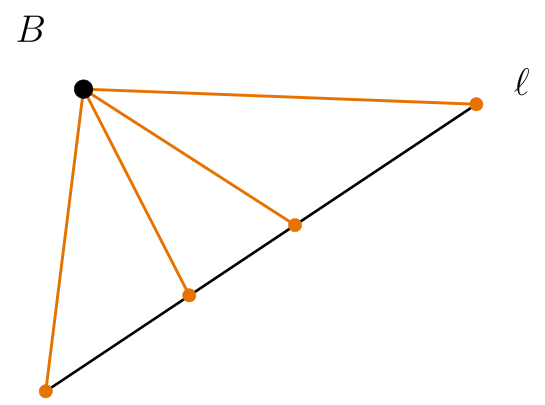
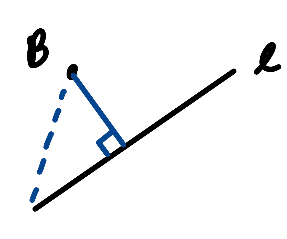
Setup: Suppose we have a line in R 2 \mathbb{R}^2 R 2 R 3 \mathbb{R}^3 R 3
Although there are many lines from B B B ℓ \ell ℓ B B B ℓ \ell ℓ B B B ℓ \ell ℓ ℓ \ell ℓ
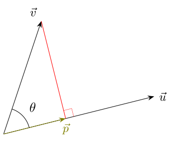
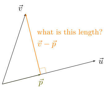
Let u ⃗ \vec{u} u v ⃗ \vec{v} v p ⃗ \vec{p} p v ⃗ \vec{v} v u ⃗ \vec{u} u p ⃗ \vec{p} p projection of v ⃗ \vec{v} v u ⃗ \vec{u} u .
Two goals:
Can we find a formula for p ⃗ \vec{p} p u ⃗ \vec{u} u v ⃗ \vec{v} v
Can we find the length of the red line?
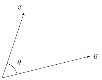
Let θ \theta θ u ⃗ \vec{u} u v ⃗ \vec{v} v
Notice that v ⃗ \vec{v} v p ⃗ \vec{p} p v ⃗ − p ⃗ \vec{v} - \vec{p} v − p p ⃗ \vec{p} p θ \theta θ v ⃗ \vec{v} v p ⃗ \vec{p} p θ \theta θ cos = adjacent / hypotenuse \cos = \text{adjacent}/\text{hypotenuse} cos = adjacent / hypotenuse
cos θ = ∥ p ⃗ ∥ ∥ v ⃗ ∥ ⟹ ∥ p ⃗ ∥ = ∥ v ⃗ ∥ cos θ (1) \cos\theta = \frac{\|\vec{p}\|}{\|\vec{v}\|} \implies \|\vec{p}\| = \|\vec{v}\|\cos\theta \tag{1} cos θ = ∥ v ∥ ∥ p ∥ ⟹ ∥ p ∥ = ∥ v ∥ cos θ ( 1 ) Let u ^ \hat{u} u ^ u ⃗ \vec{u} u u ^ \hat{u} u ^ u ⃗ \vec{u} u
u ^ = 1 ∥ u ⃗ ∥ u ⃗ (2) \hat{u} = \frac{1}{\|\vec{u}\|}\vec{u} \tag{2} u ^ = ∥ u ∥ 1 u ( 2 ) Since p ⃗ \vec{p} p u ⃗ \vec{u} u v ⃗ \vec{v} v u ^ \hat{u} u ^
p ⃗ = ∥ p ⃗ ∥ u ^ (3) \vec{p} = \|\vec{p}\|\hat{u} \tag{3} p = ∥ p ∥ u ^ ( 3 ) By chaining (1), (2), and (3), and recalling from last time that cos θ = u ⃗ T v ⃗ ∥ u ⃗ ∥ ∥ v ⃗ ∥ \cos\theta = \dfrac{\vec{u}^T\vec{v}}{\|\vec{u}\|\|\vec{v}\|} cos θ = ∥ u ∥∥ v ∥ u T v
p ⃗ = ∥ p ⃗ ∥ u ^ (3) = ∥ v ⃗ ∥ cos θ u ^ (1) = ∥ v ⃗ ∥ ⋅ u ⃗ T v ⃗ ∥ u ⃗ ∥ ∥ v ⃗ ∥ u ^ = ∥ v ⃗ ∥ ⋅ u ⃗ T v ⃗ ∥ u ⃗ ∥ ∥ v ⃗ ∥ ⋅ 1 ∥ u ⃗ ∥ u ⃗ (2) = ∥ v ⃗ ∥ ⋅ u ⃗ T v ⃗ ∥ u ⃗ ∥ ∥ v ⃗ ∥ ⋅ 1 ∥ u ⃗ ∥ u ⃗ = u ⃗ T v ⃗ ∥ u ⃗ ∥ ∥ u ⃗ ∥ u ⃗ = u ⃗ T v ⃗ ∥ u ⃗ ∥ 2 u ⃗ ( ∥ u ⃗ ∥ 2 = u ⃗ T u ⃗ ) = u ⃗ T v ⃗ u ⃗ T u ⃗ ⏟ scalar u ⃗ \begin{aligned}
\vec{p} &= \|\vec{p}\|\hat{u} && \text{(3)} \\
&= \|\vec{v}\|\cos\theta\; \hat{u} && \text{(1)} \\
&= \|\vec{v}\| \cdot \frac{\vec{u}^T\vec{v}}{\|\vec{u}\|\|\vec{v}\|}\; \hat{u} \\
&= \|\vec{v}\| \cdot \frac{\vec{u}^T\vec{v}}{\|\vec{u}\|\|\vec{v}\|} \cdot \frac{1}{\|\vec{u}\|}\vec{u} && \text{(2)} \\
&= \cancel{\|\vec{v}\|} \cdot \frac{\vec{u}^T\vec{v}}{\|\vec{u}\|\cancel{\|\vec{v}\|}} \cdot \frac{1}{\|\vec{u}\|}\vec{u} \\
&= \frac{\vec{u}^T\vec{v}}{\|\vec{u}\|\|\vec{u}\|}\vec{u} \\
&= \frac{\vec{u}^T\vec{v}}{\|\vec{u}\|^2}\vec{u} && \left(\|\vec{u}\|^2 = \vec{u}^T\vec{u}\right) \\
&= \underbrace{\frac{\vec{u}^T\vec{v}}{\vec{u}^T\vec{u}}}_{\text{scalar}}\,\vec{u}
\end{aligned} p = ∥ p ∥ u ^ = ∥ v ∥ cos θ u ^ = ∥ v ∥ ⋅ ∥ u ∥∥ v ∥ u T v u ^ = ∥ v ∥ ⋅ ∥ u ∥∥ v ∥ u T v ⋅ ∥ u ∥ 1 u = ∥ v ∥ ⋅ ∥ u ∥ ∥ v ∥ u T v ⋅ ∥ u ∥ 1 u = ∥ u ∥∥ u ∥ u T v u = ∥ u ∥ 2 u T v u = scalar u T u u T v u (3) (1) (2) ( ∥ u ∥ 2 = u T u )
If u ⃗ \vec{u} u v ⃗ \vec{v} v R n \mathbb{R}^n R n u ⃗ ≠ 0 ⃗ \vec{u} \neq \vec{0} u = 0 projection of v ⃗ \vec{v} v u ⃗ \vec{u} u is denoted by proj u ⃗ ( v ⃗ ) \text{proj}_{\vec{u}}(\vec{v}) proj u ( v )
proj u ⃗ ( v ⃗ ) ⏟ p ⃗ = ( u ⃗ T v ⃗ u ⃗ T u ⃗ ) u ⃗ \underbrace{\text{proj}_{\vec{u}}(\vec{v})}_{\vec{p}} = \left(\frac{\vec{u}^T\vec{v}}{\vec{u}^T\vec{u}}\right)\vec{u} p proj u ( v ) = ( u T u u T v ) u
Intuitively, a projection vector is your “shadow” vector. Picture a light source shining rays perpendicular to u ⃗ \vec{u} u v ⃗ \vec{v} v u ⃗ \vec{u} u p ⃗ \vec{p} p
Note that the shadow always falls on the line through u ⃗ \vec{u} u p ⃗ \vec{p} p u ⃗ \vec{u} u v ⃗ \vec{v} v u ⃗ \vec{u} u
Q: What is the length of the red segment?
The red segment can be thought of as the vector v ⃗ − p ⃗ \vec{v} - \vec{p} v − p ∥ v ⃗ − p ⃗ ∥ \|\vec{v} - \vec{p}\| ∥ v − p ∥
∥ v ⃗ − p ⃗ ∥ = ∥ v ⃗ − proj u ⃗ ( v ⃗ ) ∥ = ∥ v ⃗ − u ⃗ T v ⃗ u ⃗ T u ⃗ u ⃗ ∥ \|\vec{v} - \vec{p}\| = \left\|\vec{v} - \text{proj}_{\vec{u}}(\vec{v})\right\| = \left\|\vec{v} - \frac{\vec{u}^T\vec{v}}{\vec{u}^T\vec{u}}\,\vec{u}\right\| ∥ v − p ∥ = ∥ v − proj u ( v ) ∥ = v − u T u u T v u When it comes to linear equations, we are familiar with the following form y = m x + b y = mx + b y = m x + b general form of the equation of a line .
General form
a x + b y = c ax + by = c a x + b y = c
Slope-intercept form
y = m x + b y = mx + b y = m x + b
Note: the b b b b b b
Example: Convert 7 x + 12 y = 15 7x + 12y = 15 7 x + 12 y = 15
7 x + 12 y = 15 ⟺ 12 y = − 7 x + 15 ⟺ y = − 7 12 x + 15 12 7x + 12y = 15 \iff 12y = -7x + 15 \iff y = -\frac{7}{12}x + \frac{15}{12} 7 x + 12 y = 15 ⟺ 12 y = − 7 x + 15 ⟺ y = − 12 7 x + 12 15 The goal is to express the equation of a line entirely in terms of vectors, so that the unknowns x , y x, y x , y a , b a, b a , b
a x + b y = c a x 1 + b x 2 = c ( x → x 1 , y → x 2 ) w 1 x 1 + w 2 x 2 = c ( a → w 1 , b → w 2 ) w 1 x 1 + w 2 x 2 − c = 0 w 1 x 1 + w 2 x 2 + b = 0 ( − c → b ) \begin{aligned}
ax + by &= c \\
ax_1 + bx_2 &= c && (x \to x_1,\; y \to x_2) \\
w_1x_1 + w_2x_2 &= c && (a \to w_1,\; b \to w_2) \\
w_1x_1 + w_2x_2 - c &= 0 \\
w_1x_1 + w_2x_2 + b &= 0 && (-c \to b)
\end{aligned} a x + b y a x 1 + b x 2 w 1 x 1 + w 2 x 2 w 1 x 1 + w 2 x 2 − c w 1 x 1 + w 2 x 2 + b = c = c = c = 0 = 0 ( x → x 1 , y → x 2 ) ( a → w 1 , b → w 2 ) ( − c → b ) This can be written as a matrix product:
[ w 1 w 2 ] [ x 1 x 2 ] + b = 0 ⟹ w ⃗ T x ⃗ + b = 0 (vector equation of a 2-dimensional line) \begin{bmatrix} w_1 & w_2 \end{bmatrix} \begin{bmatrix} x_1 \\ x_2 \end{bmatrix} + b = 0
\quad\Longrightarrow\quad
\vec{w}^T\vec{x} + b = 0 \quad \text{(vector equation of a 2-dimensional line)} [ w 1 w 2 ] [ x 1 x 2 ] + b = 0 ⟹ w T x + b = 0 (vector equation of a 2-dimensional line) If w ⃗ \vec{w} w x ⃗ \vec{x} x w ⃗ = [ 2 5 7 ] \vec{w} = \begin{bmatrix} 2 \\ 5 \\ 7 \end{bmatrix} w = 2 5 7 x ⃗ = [ x 1 x 2 x 3 ] \vec{x} = \begin{bmatrix} x_1 \\ x_2 \\ x_3 \end{bmatrix} x = x 1 x 2 x 3 b = 3 b = 3 b = 3 w ⃗ T x ⃗ + b = 0 \vec{w}^T\vec{x} + b = 0 w T x + b = 0
[ 2 5 7 ] [ x 1 x 2 x 3 ] + 3 = 0 ⟺ 2 x 1 + 5 x 2 + 7 x 3 + 3 = 0 (equation of a plane) \begin{bmatrix} 2 & 5 & 7 \end{bmatrix} \begin{bmatrix} x_1 \\ x_2 \\ x_3 \end{bmatrix} + 3 = 0
\iff
2x_1 + 5x_2 + 7x_3 + 3 = 0 \quad \text{(equation of a plane)} [ 2 5 7 ] x 1 x 2 x 3 + 3 = 0 ⟺ 2 x 1 + 5 x 2 + 7 x 3 + 3 = 0 (equation of a plane)
In 2D, w ⃗ T x ⃗ + b = 0 \vec{w}^T\vec{x} + b = 0 w T x + b = 0
In 3D, w ⃗ T x ⃗ + b = 0 \vec{w}^T\vec{x} + b = 0 w T x + b = 0
In general (in R n \mathbb{R}^n R n n n n w ⃗ T x ⃗ + b = 0 \vec{w}^T\vec{x} + b = 0 w T x + b = 0 hyperplane .
Hyperplanes sound scary/fancy, but this is just a generalization of a 2D line.
For every hyperplane w ⃗ T x ⃗ + b = 0 \vec{w}^T\vec{x} + b = 0 w T x + b = 0 w ⃗ \vec{w} w
Proof
Take any two points x ⃗ 1 \vec{x}_1 x 1 x ⃗ 2 \vec{x}_2 x 2 w ⃗ T x ⃗ 1 + b = 0 \vec{w}^T\vec{x}_1 + b = 0 w T x 1 + b = 0 w ⃗ T x ⃗ 2 + b = 0 \vec{w}^T\vec{x}_2 + b = 0 w T x 2 + b = 0
w ⃗ T x ⃗ 2 − w ⃗ T x ⃗ 1 = 0 ⟹ w ⃗ T ( x ⃗ 2 − x ⃗ 1 ) = 0 \vec{w}^T\vec{x}_2 - \vec{w}^T\vec{x}_1 = 0 \implies \vec{w}^T(\vec{x}_2 - \vec{x}_1) = 0 w T x 2 − w T x 1 = 0 ⟹ w T ( x 2 − x 1 ) = 0 So w ⃗ \vec{w} w x ⃗ 2 − x ⃗ 1 \vec{x}_2 - \vec{x}_1 x 2 − x 1 w ⃗ \vec{w} w