Lec 05-05-2026: Support Vector Machines: Motivation & Setup

Wisconsin Breast Cancer Dataset

Last lecture we sketched a subset of the Wisconsin Breast Cancer Dataset.

Notation: $x^i_j$ where $i$ = patient #, $j$ = feature #

$Two patients (1 and 569) represented as stick figures, each with a box listing their tumor features and labels$

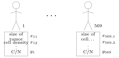
Since the output is not numeric, let’s perform a conversion:

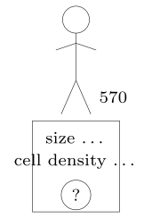
y_i = \begin{cases} -1 & \text{if person } i \text{ has no cancer} \\ +1 & \text{if person } i \text{ has cancer} \end{cases}

$Patient 570 as a stick figure with a feature box showing size, cell density, and an unknown label (?)$

A new patient 570 walks in with features (size…, cell density…, …) but with an unknown label.

The Classification Question

Q: A new patient walks in with a tumor. Can we predict if the tumor is/isn’t cancerous?

Q: Can we come up with a line (hyperplane) that does a good job at separating these two classes?

A: We answered this (fully) in 1994.

It is tough to draw a separating line because every line/hyperplane will misclassify some points.

Since this question is hard:

We will pose an easier question
We will investigate if the easier question happens IRL
We will try to answer the easier question
We will try to modify our answer to answer the harder question

Phase 1: Pose an Easier Question

Since every line/hyperplane misclassifies some things, it would be easier if our dataset looked like:

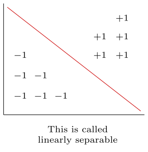
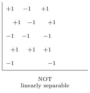
$Scatter plot with -1 points in the lower-left and +1 points in the upper-right, separated by a red diagonal hyperplane, labeled 'This is called linearly separable'$

$Scatter plot with +1 and -1 points randomly mixed with no discernible pattern, labeled 'NOT linearly separable'$

Def. A set of points is said to be linearly separable if there exists a hyperplane such that one side of the hyperplane consists of all points with label $-1$ and the other side contains all points with label $+1$ .

Q: If the data is linearly separable, how many hyperplanes can we draw?

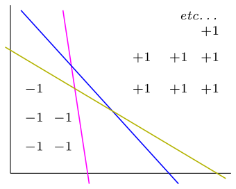
$Scatter plot with -1 and +1 points showing three valid separating hyperplanes drawn in pink, blue, and yellow$

There are infinitely many hyperplanes.

Q: Which is the “best”?

A: The support vector machine gives one way of finding the “best” hyperplane.

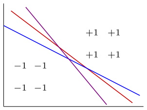
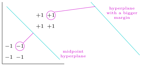
The Best Hyperplane

The idea is this. Consider the following 2 hyperplanes imposed upon the same dataset:

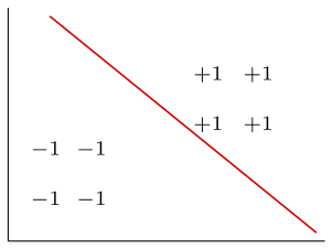
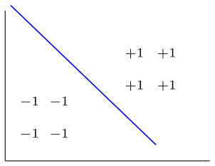
$Scatter plot with a red hyperplane that has a small margin, positioned close to the data points$

$Scatter plot with a blue hyperplane that has a large margin, positioned centrally between the two clusters$

Claim: The blue hyperplane will generalize better.

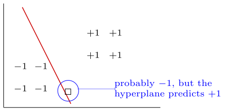
$Scatter plot with red hyperplane, a new borderline square point misclassified as +1 by the hyperplane, with annotation 'probably -1, but the hyperplane predicts +1'$

The blue hyperplane has more “breathing room” — there is a larger margin between the hyperplane and the surrounding points.

We care about maximizing the distance from the hyperplane to the nearest point, i.e. maximizing the margin.

\text{margin} = \min(1, 5) = 1

$Scatter plot with a red hyperplane positioned close to the -1 cluster; the nearest -1 point (circled) has a short distance (labeled 1) to the hyperplane and the nearest +1 point (circled, far away) has a long distance (labeled 5) to the hyperplane$

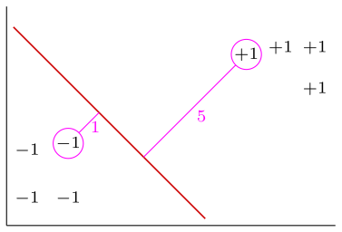
Our goal is to maximize the margin. SVM will tell us how to do this.

The Easier Question

In a linearly separable dataset, how can we find the hyperplane which maximizes the margin?

The hyperplane equation is:

\vec{w}^T \vec{x} + b = 0

We want to find $\vec{w}$ and $b$ .

Here, $\vec{x}$ is the feature vector of a data point (the inputs), while $\vec{w}$ and $b$ are the unknowns that define the hyperplane - $\vec{w}$ controls its orientation and $b$ controls its offset from the origin.

Phase 2: Does Linearly Separable Data Happen IRL?

If the # of dimensions is low, no
If the # of dimensions is high, it likely is linearly separable

2 reasons for this:

Higher dimensional spaces are “roomier” (more space, so more likely to separate the data)

Think of being stuck in traffic: in 2D (the road), everyone is clustered and impossible to separate. But introduce a third dimension - the ability to fly - and you can lift some cars up and pass a plane between them. The same idea applies to data: more dimensions give the hyperplane more directions to orient itself, making it easier to slip one between the two classes.
Blessing of non-uniformity - the phenomenon is sometimes not random
- Ex. If cancer was random, we would see this:

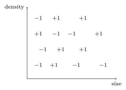
$Scatter plot with density (vertical) and size (horizontal) axes; +1 and -1 labels randomly mixed with no discernible pattern$

If data were truly random, you couldn’t make predictions - no pattern to exploit, no clustering to speak of. It would be like throwing darts at a board. But IRL we see:

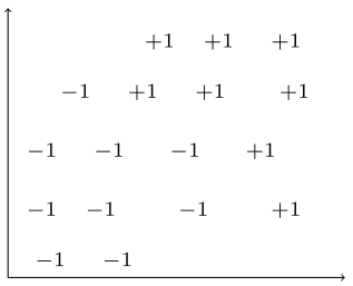
$Scatter plot where -1 points are concentrated in the lower-left and +1 points in the upper-right, with some intermixing near the middle boundary$

Datapoints are often concentrated in a specific region.

Phase 3: Finding the Optimal Hyperplane

Given a linearly separable dataset, how can we find the hyperplane which maximizes the margin?

We first define what is meant by “margin.”

Def. Given a dataset $\mathbb{D}$ of the form $\mathbb{D} = \{(\vec{x}_i, y_i) \mid y_i \in \{-1, 1\}\}$ , we define the margin of the hyperplane corresponding to $\vec{w}^T \vec{x} + b = 0$ , denoted by

\gamma(\vec{w}, b) := \min_{\vec{x}_i \in \mathbb{D}} \frac{\lvert \vec{w}^T \vec{x}_i + b \rvert}{\lVert \vec{w} \rVert}

The expression $\frac{\lvert \vec{w}^T \vec{x}_i + b \rvert}{\lVert \vec{w} \rVert}$ is the perpendicular distance from point $\vec{x}_i$ to the hyperplane $\vec{w}^T \vec{x} + b = 0$ - a result from linear algebra (the projection distance formula).

The formula works as follows:

For each point in our training data
Compute the distance from the point to the hyperplane
Take the minimum distance

The formula tells us how to find the margin given a hyperplane & a set of points.

As mentioned previously, our goal is to find the $\vec{w}$ & $b$ which maximizes $\gamma(\vec{w}, b)$ :

Goal:

\underset{\vec{w},\, b}{\arg\max} \; \gamma(\vec{w}, b)

Each part of this expression has a specific role:

$\arg\max$ (the operator): “Return the argument that produces the maximum, not the maximum value itself.” Contrast with plain $\max$ : if $f(5) = 20$ is the peak, then $\max f = 20$ but $\arg\max f = 5$ .
$\vec{w}, b$ (the subscript): What you are free to vary in the search - all possible choices of $\vec{w}$ and $b$ , i.e. all possible hyperplanes. These are the unknowns you want to find.
$\gamma(\vec{w}, b)$ (the expression): The thing being maximized - the margin as a function of the hyperplane. For any given $\vec{w}$ and $b$ , this evaluates to the size of that hyperplane’s margin.

Put together: “Among all choices of $\vec{w}$ and $b$ , find the ones that make the margin $\gamma(\vec{w}, b)$ as large as possible.”

Original Explanation:

The notation $\arg\max$ means “return the input that produces the maximum, not the maximum value itself.” For example, if $f(5) = 20$ is the maximum of $f$ , then $\max f = 20$ but $\arg\max f = 5$ . Here we want the specific $\vec{w}$ and $b$ that yield the largest margin - not the margin value itself.

$Scatter plot with -1 and +1 points showing three valid separating hyperplanes drawn in red, blue, and purple$

To compute $\underset{\vec{w},b}{\arg\max} \; \gamma(\vec{w},b)$ :

Search through each hyperplane
Compute the margin associated to each hyperplane
Return the $\vec{w}$ and $b$ that produce the maximum margin

$Two panels: left shows midpoint hyperplane separating -1 cluster (lower-left, one circled) and +1 cluster (upper-right, one circled); right shows a larger-margin hyperplane far from the data$

A Problem with This Formulation

There is a subtle issue with the goal as stated. If we simply ask a computer to find the $\vec{w}$ and $b$ that maximize $\gamma(\vec{w}, b)$ , it will push the hyperplane off to infinity.

Why? Because $\gamma(\vec{w}, b)$ is the minimum distance from the hyperplane to any data point. If we slide the hyperplane far away from all the data, that minimum distance keeps growing - there is nothing in the formulation that prevents it. The computer would happily report a margin of 342, then 1000, then $\infty$ .

To fix this, we need to add a constraint that keeps the hyperplane anchored near the data. This turns the problem into a constrained optimization - the same kind encountered in calculus when maximizing the area of a garden subject to a limited amount of fencing material:

\underset{\vec{w},\, b}{\arg\max} \; \gamma(\vec{w}, b) \quad \text{subject to a constraint on } \vec{w}, b

Choosing the right constraint, and then simplifying the resulting problem, is what comes next.