Midterm 1 Review: Sequential Sequence Problems

Original Document: Type of problems for Midterm 1 (Partial Solutions)

Topics covered on the exam

• Design problems using f/f
  • Counters
  • Self-correcting circuits
  • State tables, state diagrams, and circuit diagrams
• Master-Slave Flip-Flop
  • Given the clock and input signals in a timing diagram, determine the output of the master and slave f/f
• Be familiar with shift registers and general registers

Must know the characteristic tables for the different flip-flop types. You will be given the excitation tables.

Problem 1: Designing a Traffic Light

Design a Traffic Light using D Flip-Flops. Define 6 states (000 — 101):

state 0 (R/R) $\to$ state 1 (G/R) $\to$ state 2 (Y/R) $\to$ state 3 (R/R) $\to$ state 4 (R/G) $\to$ state 5 (R/Y)

 

Problem 2: Traffic Light with Emergency State

Extend Problem 1 by adding an emergency state:

• RY blink:
  • for $x = 1$: go into emergency state
  • for $x = 0$: go into next state

Consider the emergency state to be 110. We now have 7 states (0 to 6) and a 4-variable table for ABC and X. From the emergency state, $x=1$ stays in emergency and $x=0$ resets to 000. You can also consider that by 0/1 stays in the emergency state — in that case you will get different expressions for the f/f inputs.

 

Problem 3: Sequential Circuit with Two D Flip-Flops

A sequential circuit with two D f/f, $A$ and $B$; two inputs, $x$ and $y$; and one output $Z$ is specified by the following next-state and output functions:

$$\begin{aligned} A(t+1) &= x'y + xA \\ B(t+1) &= x'B + xA \\ Z &= B \end{aligned}$$

• Draw the circuit
• Derive the state table
• Derive the state diagram

Solution

Draw the state table:

$$\begin{array}{cc|cc|cc|c} Q(t) & & \text{Inputs} & & Q(t{+}1) & & \text{Output} \\ \hline A & B & x & y & A & B & Z \\ \hline 0 & 0 & 0 & 0 & & & \\ 0 & 0 & 0 & 1 & & & \\ 0 & 0 & 1 & 0 & & & \\ 0 & 0 & 1 & 1 & & & \\ 0 & 1 & 0 & 0 & & & \\ 0 & 1 & 0 & 1 & & & \\ 0 & 1 & 1 & 0 & & & \\ 0 & 1 & 1 & 1 & & & \\ 1 & 0 & 0 & 0 & & & \\ 1 & 0 & 0 & 1 & & & \\ 1 & 0 & 1 & 0 & & & \\ 1 & 0 & 1 & 1 & & & \\ 1 & 1 & 0 & 0 & & & \\ 1 & 1 & 0 & 1 & & & \\ 1 & 1 & 1 & 0 & & & \\ 1 & 1 & 1 & 1 & & & \\ \end{array}$$

Since we’re given the next-state functions directly, we can evaluate $A(t+1)$, $B(t+1)$, and $Z$ for each row by substituting the present state and inputs:

$$\begin{array}{cc|cc|cc|c} Q(t) & & \text{Inputs} & & Q(t{+}1) & & \text{Output} \\ \hline A & B & x & y & A & B & Z \\ \hline 0 & 0 & 0 & 0 & 0 & 0 & 0 \\ 0 & 0 & 0 & 1 & 1 & 0 & 0 \\ 0 & 0 & 1 & 0 & 0 & 0 & 0 \\ 0 & 0 & 1 & 1 & 0 & 0 & 0 \\ 0 & 1 & 0 & 0 & 0 & 1 & 1 \\ 0 & 1 & 0 & 1 & 1 & 1 & 1 \\ 0 & 1 & 1 & 0 & 0 & 0 & 1 \\ 0 & 1 & 1 & 1 & 0 & 0 & 1 \\ 1 & 0 & 0 & 0 & 0 & 0 & 0 \\ 1 & 0 & 0 & 1 & 1 & 0 & 0 \\ 1 & 0 & 1 & 0 & 1 & 1 & 0 \\ 1 & 0 & 1 & 1 & 1 & 1 & 0 \\ 1 & 1 & 0 & 0 & 0 & 1 & 1 \\ 1 & 1 & 0 & 1 & 1 & 1 & 1 \\ 1 & 1 & 1 & 0 & 1 & 1 & 1 \\ 1 & 1 & 1 & 1 & 1 & 1 & 1 \\ \end{array}$$

Draw the state diagram:

Each of the four present states $AB$ becomes a node. Since there are two inputs $x$ and $y$, each state has four outgoing edges labeled $xy/Z$:

Drawing the circuit:

In general, drawing the circuit requires knowing the f/f input expressions. You would derive them by filling in the $D_A$ and $D_B$ columns of the state table using the D flip-flop excitation table, then working through the K-maps to derive the minimized expressions.

In this problem, however, the next-state functions $A(t+1)$ and $B(t+1)$ are given directly. Because a D flip-flop passes its input straight through to its output — that is, $D = Q(t+1)$ — the next-state function and the D input expression are one and the same. So the next-state expressions from the problem statement can be used directly as the D input expressions:

$$D_A = x'y + xA \qquad D_B = x'B + xA$$

 

Problem 4: Full Adder Connected to a D Flip-Flop

A sequential circuit has one f/f $Q$; two inputs, $x$ and $y$; and one output $S$. It consists of a full adder circuit connected to a D f/f. Derive the state table and state diagram of the sequential circuit.

 

Problem 5: Self-Correcting Sequential Circuit Design

A sequential circuit has three f/f $A$, $B$, $C$; one input $x$; one output $y$.

• Design the circuit using D f/f, treating unused states as don’t care conditions
• Analyze if the circuit is self-correcting

Solution

Draw the state table:

The state diagram tells us plenty of information upfront: the valid states, invalid states (the missing states), $x$ input values that drive the transition for each state, and the output $y$ for each transition. Using that information, we fill the state table (the unused states can optionally be included, filled in as Don’t Cares):

$$\begin{array}{ccc|c|ccc|ccc|c} & Q(t) & & \text{Input} & & Q(t{+}1) & & \text{f/f} & \text{Inputs} & & \text{Output} \\ \hline A & B & C & x & A & B & C & D_A & D_B & D_C & y \\ \hline 0 & 0 & 0 & 0 & 0 & 1 & 1 & & & & 0 \\ 0 & 0 & 0 & 1 & 1 & 0 & 0 & & & & 1 \\ 0 & 0 & 1 & 0 & 0 & 0 & 1 & & & & 0 \\ 0 & 0 & 1 & 1 & 1 & 0 & 0 & & & & 1 \\ 0 & 1 & 0 & 0 & 0 & 1 & 0 & & & & 0 \\ 0 & 1 & 0 & 1 & 0 & 0 & 0 & & & & 1 \\ 0 & 1 & 1 & 0 & 0 & 0 & 1 & & & & 0 \\ 0 & 1 & 1 & 1 & 0 & 1 & 0 & & & & 1 \\ 1 & 0 & 0 & 0 & 0 & 1 & 0 & & & & 0 \\ 1 & 0 & 0 & 1 & 0 & 1 & 1 & & & & 0 \\ \color{red}1 & \color{red}0 & \color{red}1 & 0 & X & X & X & X & X & X & X \\ \color{red}1 & \color{red}0 & \color{red}1 & 1 & X & X & X & X & X & X & X \\ \color{red}1 & \color{red}1 & \color{red}0 & 0 & X & X & X & X & X & X & X \\ \color{red}1 & \color{red}1 & \color{red}0 & 1 & X & X & X & X & X & X & X \\ \color{red}1 & \color{red}1 & \color{red}1 & 0 & X & X & X & X & X & X & X \\ \color{red}1 & \color{red}1 & \color{red}1 & 1 & X & X & X & X & X & X & X \\ \end{array}$$

Fill in the f/f inputs

Use the D flip-flop excitation table to determine the specific values of $D_A$, $D_B$, $D_C$ that will produce the next state values:

$$\begin{array}{cc|c} Q(t) & Q(t+1) & D \\ \hline 0 & 0 & 0 \\ 0 & 1 & 1 \\ 1 & 0 & 0 \\ 1 & 1 & 1 \\ \end{array}$$ $$\begin{array}{ccc|c|ccc|ccc|c} & Q(t) & & \text{Input} & & Q(t{+}1) & & \text{f/f} & \text{Inputs} & & \text{Output} \\ \hline A & B & C & x & A & B & C & D_A & D_B & D_C & y \\ \hline 0 & 0 & 0 & 0 & 0 & 1 & 1 & 0 & 1 & 1 & 0 \\ 0 & 0 & 0 & 1 & 1 & 0 & 0 & 1 & 0 & 0 & 1 \\ 0 & 0 & 1 & 0 & 0 & 0 & 1 & 0 & 0 & 1 & 0 \\ 0 & 0 & 1 & 1 & 1 & 0 & 0 & 1 & 0 & 0 & 1 \\ 0 & 1 & 0 & 0 & 0 & 1 & 0 & 0 & 1 & 0 & 0 \\ 0 & 1 & 0 & 1 & 0 & 0 & 0 & 0 & 0 & 0 & 1 \\ 0 & 1 & 1 & 0 & 0 & 0 & 1 & 0 & 0 & 1 & 0 \\ 0 & 1 & 1 & 1 & 0 & 1 & 0 & 0 & 1 & 0 & 1 \\ 1 & 0 & 0 & 0 & 0 & 1 & 0 & 0 & 1 & 0 & 0 \\ 1 & 0 & 0 & 1 & 0 & 1 & 1 & 0 & 1 & 1 & 0 \\ \color{red}1 & \color{red}0 & \color{red}1 & 0 & X & X & X & X & X & X & X \\ \color{red}1 & \color{red}0 & \color{red}1 & 1 & X & X & X & X & X & X & X \\ \color{red}1 & \color{red}1 & \color{red}0 & 0 & X & X & X & X & X & X & X \\ \color{red}1 & \color{red}1 & \color{red}0 & 1 & X & X & X & X & X & X & X \\ \color{red}1 & \color{red}1 & \color{red}1 & 0 & X & X & X & X & X & X & X \\ \color{red}1 & \color{red}1 & \color{red}1 & 1 & X & X & X & X & X & X & X \\ \end{array}$$

Derive the flip-flop input expressions:

Unused states ABC = 101, 110, 111 treated as Don’t Care conditions on the K-maps:

$D_A:$

$$D_A = A'B'x$$

$D_B:$

$$D_B = C'x' + A + BCx$$

$D_C:$

$$D_C = A'B'x' + Cx' + Ax$$

$y:$

$$y = A'x$$

Check for self-correction:

We plug each unused state into the derived expressions and trace where the circuit goes next.

Unused state ABC = 101:

$$\begin{aligned} D_A &= A'B'x = 0 & &\Rightarrow A \text{ reset to } 0 \\ D_B &= C'x' + A + BCx = 0 + 1 + 0 = 1 & &\Rightarrow B \text{ set to } 1 \\ D_C &= A'B'x' + Cx' + Ax = 0 + x' + x = 1 & &\Rightarrow C \text{ set to } 1 \end{aligned}$$ $$101 \to 011$$

State 011 is valid, so the circuit self-corrects out of state 101.

Unused state ABC = 110:

$$\begin{aligned} D_A &= A'B'x = 0 & &\Rightarrow A \text{ reset to } 0 \\ D_B &= C'x' + A + BCx = x' + 1 + 0 = 1 & &\Rightarrow B \text{ set to } 1 \\ D_C &= A'B'x' + Cx' + Ax = 0 + 0 + x = x & & \Rightarrow C \text{ dependent on } x \\ \end{aligned}$$ $$110 \to 01?$$

Invalid state 110 could transition to either of two states, so now we check the two cases:

• $x = 0$:

$$D_C = x = 0 \quad\Rightarrow\quad C \text{ reset to } 0$$ $$110 \xrightarrow{0} 010$$

• $x = 1$:

$$D_C = x = 1 \quad\Rightarrow\quad C \text{ set to } 1$$ $$110 \xrightarrow{1} 011$$

Both states 010 and 011 are valid, so the circuit self-corrects out of state 110.

Unused state ABC = 111:

$$\begin{aligned} D_A &= A'B'x = 0 & &\Rightarrow A \text{ reset to } 0 \\ D_B &= C'x' + A + BCx = 0 + 1 + x = 1 & &\Rightarrow B \text{ set to } 1 \\ D_C &= A'B'x' + Cx' + Ax = 0 + x' + x = 1 & &\Rightarrow C \text{ set to } 1 \end{aligned}$$ $$111 \to 011$$

State 011 is valid, so the circuit self-corrects out of state 111.

All unused states transition to valid states regardless of input, so the circuit is self-correcting.

Note

On the exam, you may be asked to analyze only one of the unused states for self-correction due to time constraints.

 

Problem 6: JK Flip-Flop Sequential Circuit

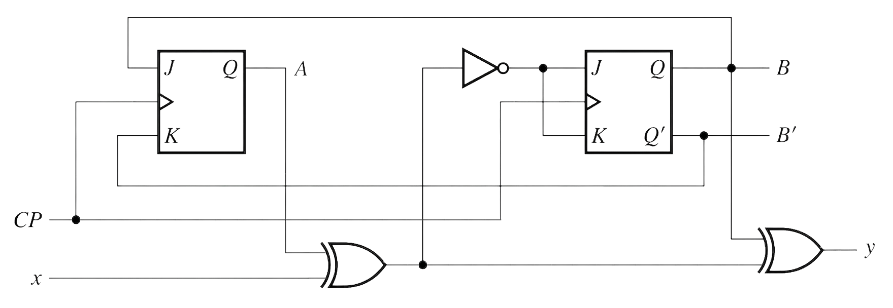
A sequential circuit has 2 JK f/f, one input $x$, and one output $y$. The logic diagram is shown below. Derive the state table and state diagram.

Solution

Get the expression of the f/f inputs (based on present states and external input) by tracing through the given circuit diagram. Based on present state and f/f inputs, get the next state.

f/f input and $y$ output expressions:

$$\begin{aligned} J_A &= B & \qquad J_B &= (x \oplus A)' \\ K_A &= B' & \qquad K_B &= (x \oplus A)' \end{aligned}$$ $$y = x \oplus A \oplus B$$

Draw the state table:

$$\begin{array}{cc|c|cc|cccc|c} Q(t) & & \text{Input} & Q(t{+}1) & & \text{f/f} & \text{Inputs} & & & Output \\ \hline A & B & x & A & B & J_A & K_A & J_B & K_B & y \\ \hline 0 & 0 & 0 & & & & & & & \\ 0 & 0 & 1 & & & & & & & \\ 0 & 1 & 0 & & & & & & & \\ 0 & 1 & 1 & & & & & & & \\ 1 & 0 & 0 & & & & & & & \\ 1 & 0 & 1 & & & & & & & \\ 1 & 1 & 0 & & & & & & & \\ 1 & 1 & 1 & & & & & & & \\ \end{array}$$

Fill in the flip-flop inputs:

The f/f inputs and the $y$ output are the first thing we can compute, since they depend only on the present state and $x$, which we already have.

$$\begin{array}{cc|c|cc|cccc|c} Q(t) & & \text{Input} & Q(t{+}1) & & \text{f/f} & \text{Inputs} & & & Output \\ \hline A & B & x & A & B & J_A & K_A & J_B & K_B & y \\ \hline 0 & 0 & 0 & & & 0 & 1 & 1 & 1 & 0 \\ 0 & 0 & 1 & & & 0 & 1 & 0 & 0 & 1 \\ 0 & 1 & 0 & & & 1 & 0 & 1 & 1 & 1 \\ 0 & 1 & 1 & & & 1 & 0 & 0 & 0 & 0 \\ 1 & 0 & 0 & & & 0 & 1 & 0 & 0 & 1 \\ 1 & 0 & 1 & & & 0 & 1 & 1 & 1 & 0 \\ 1 & 1 & 0 & & & 1 & 0 & 0 & 0 & 0 \\ 1 & 1 & 1 & & & 1 & 0 & 1 & 1 & 1 \\ \end{array}$$

Determine the next state:

With the f/f inputs in hand, each flip-flop’s next state follows from how a JK flip-flop behaves in response to its J/K inputs, as described by the JK characteristic table:

$$\begin{array}{cc|c} J & K & Q(t+1) \\ \hline 0 & 0 & Q(t) \\ 0 & 1 & 0 \\ 1 & 0 & 1 \\ 1 & 1 & Q'(t) \\ \end{array}$$

Fill in the next state values:

$$\begin{array}{cc|c|cc|cccc|c} Q(t) & & \text{Input} & Q(t{+}1) & & \text{f/f} & \text{Inputs} & & & Output \\ \hline A & B & x & A & B & J_A & K_A & J_B & K_B & y \\ \hline 0 & 0 & 0 & 0 & 1 & 0 & 1 & 1 & 1 & 0 \\ 0 & 0 & 1 & 0 & 0 & 0 & 1 & 0 & 0 & 1 \\ 0 & 1 & 0 & 1 & 0 & 1 & 0 & 1 & 1 & 1 \\ 0 & 1 & 1 & 1 & 1 & 1 & 0 & 0 & 0 & 0 \\ 1 & 0 & 0 & 0 & 0 & 0 & 1 & 0 & 0 & 1 \\ 1 & 0 & 1 & 0 & 1 & 0 & 1 & 1 & 1 & 0 \\ 1 & 1 & 0 & 1 & 1 & 1 & 0 & 0 & 0 & 0 \\ 1 & 1 & 1 & 1 & 0 & 1 & 0 & 1 & 1 & 1 \\ \end{array}$$

State Diagram:

Draw the state diagram based on the state table. Each of the four present states AB becomes a node with a directed edge leading to the next state. The edges are labeled in the form x/y, where $x$ is the input driving the transition and $y$ is the resulting output: